Kullback–Leibler Divergence

How different are two probability distributions? The Kullback–Leibler (KL) divergence answers this with the average log-ratio of the two, and that single quantity turns out to sit underneath a remarkable amount of statistics: fitting a model by maximum likelihood minimizes it, variational inference and the variational autoencoder minimize it, cross-entropy loss is it, and the log score for forecasts is built from it. It measures information — the extra surprise you suffer when you model reality with the wrong distribution — and it is famously asymmetric, which is not a defect but the source of much of its usefulness.

Definition#

For two distributions $P$ and $Q$ over the same outcomes, the KL divergence of $Q$ from $P$ is the expectation under $P$ of the log-ratio $\log\frac{P}{Q}$: $$D_{\mathrm{KL}}(P \,\|\, Q) = \sum_{x} P(x)\,\log\frac{P(x)}{Q(x)} = \mathbb{E}_{P}\!\left[\log\frac{P(x)}{Q(x)}\right], \tag{1}$$ with the sum replaced by an integral for continuous distributions. Read it as a weighted average: at each outcome, $\log\frac{P(x)}{Q(x)}$ is how much more (or less) probable that outcome is under $P$ than under $Q$, and we average those log-ratios weighting by how often $P$ actually produces the outcome. The units are nats with the natural log and bits with $\log_2$. By convention $0\log\frac{0}{q}=0$, but if $Q(x)=0$ where $P(x)>0$ the divergence is infinite — $Q$ can never rule out something $P$ considers possible.

Properties#

Three properties define its character.

• Non-negativity. $D_{\mathrm{KL}}(P\|Q)\ge 0$ always, a consequence of Jensen’s inequality applied to the concave logarithm (this is Gibbs’ inequality).
• Zero iff identical. $D_{\mathrm{KL}}(P\|Q)=0$ exactly when $P=Q$ everywhere, so it behaves like a “distance to the truth” that bottoms out at zero.
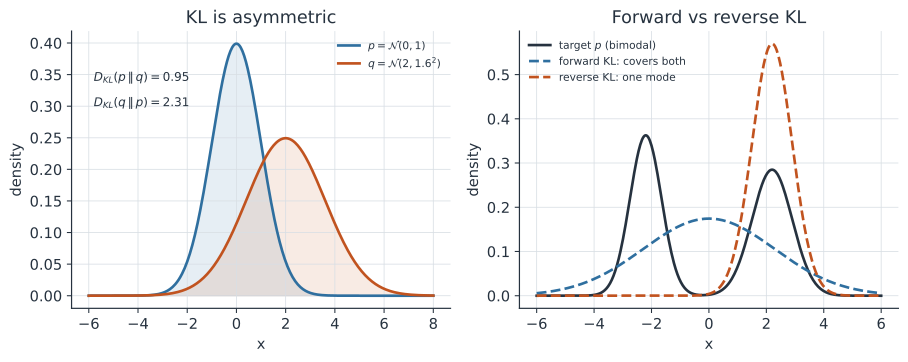
• Asymmetry. In general $D_{\mathrm{KL}}(P\|Q)\ne D_{\mathrm{KL}}(Q\|P)$, as the left panel of the figure shows.

That last point means KL is not a metric: besides being asymmetric it fails the triangle inequality. When a symmetric measure is needed, the Jensen–Shannon divergence — the average of the two directions against their mixture — is the usual symmetrized cousin.

Information interpretation#

KL divergence is relative entropy, and it slots neatly between entropy and cross-entropy. The entropy $H(P)=-\sum_x P(x)\log P(x)$ is the average surprise (optimal code length) of $P$, and the cross-entropy $H(P,Q)=-\sum_x P(x)\log Q(x)$ is the average surprise you pay when the data are really $P$ but you encode them as if they were $Q$. Their difference is exactly the divergence, $$H(P,Q) = H(P) + D_{\mathrm{KL}}(P\,\|\,Q), \tag{2}$$ so $D_{\mathrm{KL}}(P\|Q)$ is the number of extra bits wasted by using the wrong model $Q$ instead of the true $P$. This is why minimizing cross-entropy loss — the standard classification objective, including for neural networks — is minimizing KL divergence to the data-generating distribution: the entropy term $H(P)$ does not depend on the model, so it drops out of the gradient.

Forward versus reverse KL#

Because KL is asymmetric, which direction you minimize matters, and the two choices behave differently when the approximating family cannot match the target exactly — the right panel of the figure. Minimizing the forward KL $D_{\mathrm{KL}}(p\,\|\,q)$ over $q$ is mean-seeking (or mode-covering): the $p$-weighted average in (1) punishes any outcome where $p$ is large but $q$ is small, so $q$ stretches to put mass wherever $p$ does, covering all the modes and often the gaps between them. Minimizing the reverse KL $D_{\mathrm{KL}}(q\,\|\,p)$ is mode-seeking: the average is now weighted by $q$, which is heavily penalized for putting mass where $p$ is near zero, so $q$ retreats onto a single mode and stays compact. Variational inference and the VAE minimize the reverse KL between the approximate posterior $q$ and the true one, which is tractable but tends to underestimate posterior spread — a bias worth remembering when reading its uncertainty.

The Gaussian case and the VAE#

For two univariate Gaussians the divergence is closed-form, $$D_{\mathrm{KL}}\!\left(\mathcal{N}(\mu_0,\sigma_0^2)\,\|\,\mathcal{N}(\mu_1,\sigma_1^2)\right) = \log\frac{\sigma_1}{\sigma_0} + \frac{\sigma_0^2 + (\mu_0-\mu_1)^2}{2\sigma_1^2} - \frac12,$$ and the special case against a standard normal $\mathcal{N}(0,1)$ collapses to $$D_{\mathrm{KL}}\!\left(\mathcal{N}(\mu,\sigma^2)\,\|\,\mathcal{N}(0,1)\right) = \tfrac12\!\left(\mu^2 + \sigma^2 - \log\sigma^2 - 1\right).$$ This is exactly the regularizer in the VAE’s ELBO: it is the closed form that lets the encoder be penalized, in one cheap expression, for placing each input’s latent code away from the prior.

Where else it appears#

• Maximum likelihood. Fitting a model by maximum likelihood is, in the large-sample limit, minimizing $D_{\mathrm{KL}}(P_{\text{data}}\,\|\,P_\theta)$ — the model is pulled toward the true distribution.
• Mutual information. The mutual information between two variables is the KL divergence between their joint distribution and the product of their marginals, measuring how far they are from independent.
• Forecast scoring. The expected logarithmic score of a probabilistic forecast decomposes into entropy plus a KL term, which is why the log score is proper — it is optimized by reporting the true distribution.
• Model selection. The Akaike Information Criterion (AIC) is derived as an estimate of the expected KL divergence between the fitted model and the truth, so choosing the lowest-AIC model is choosing the one closest to reality in the KL sense.
• Experimental design. The expected information gain a study will provide is a KL divergence between the posterior and the prior, the objective behind Bayesian optimal design.

A worked example#

Take a three-category outcome — mild, moderate, severe — with a true distribution $P=(0.7, 0.2, 0.1)$ and a model $Q=(0.5, 0.3, 0.2)$. The forward divergence is $$D_{\mathrm{KL}}(P\|Q) = 0.7\log\tfrac{0.7}{0.5} + 0.2\log\tfrac{0.2}{0.3} + 0.1\log\tfrac{0.1}{0.2} = 0.235 - 0.081 - 0.069 = 0.085\ \text{nats}.$$ Swapping the roles gives $D_{\mathrm{KL}}(Q\|P) = 0.5\log\tfrac{0.5}{0.7} + 0.3\log\tfrac{0.3}{0.2} + 0.2\log\tfrac{0.2}{0.1} = 0.092$ nats — close here, but genuinely different, confirming the asymmetry. Both are small and positive, as they must be for two similar distributions.

In code#

Python#

import numpy as np
from scipy.stats import entropy

# a three-category outcome: true P vs model Q
P = np.array([0.7, 0.2, 0.1])
Q = np.array([0.5, 0.3, 0.2])
kl_pq = np.sum(P * np.log(P / Q))          # forward, in nats
kl_qp = np.sum(Q * np.log(Q / P))          # reverse
print(f"D_KL(P||Q) = {kl_pq:.4f} nats")
print(f"D_KL(Q||P) = {kl_qp:.4f} nats   (asymmetric)")
print(f"scipy.stats.entropy(P, Q) = {entropy(P, Q):.4f}")   # same as forward

# Gaussian closed form, and the VAE's N(mu, s^2) || N(0,1) special case
def kl_gauss(m0, s0, m1, s1):
    return np.log(s1 / s0) + (s0 ** 2 + (m0 - m1) ** 2) / (2 * s1 ** 2) - 0.5
mu, s = 1.0, 0.5
print(f"N(1,0.5^2) || N(0,1) = {kl_gauss(mu, s, 0, 1):.4f} nats")
print(f"VAE KL term 0.5(mu^2+s^2-log s^2-1) = {0.5*(mu**2+s**2-np.log(s**2)-1):.4f}")

D_KL(P||Q) = 0.0851 nats
D_KL(Q||P) = 0.0920 nats   (asymmetric)
scipy.stats.entropy(P, Q) = 0.0851
N(1,0.5^2) || N(0,1) = 0.8181 nats
VAE KL term 0.5(mu^2+s^2-log s^2-1) = 0.8181

R#

# philentropy::KL, or a direct formula; entropy::KL.plugin for counts.
library(philentropy)
P <- c(0.7, 0.2, 0.1)
Q <- c(0.5, 0.3, 0.2)
KL(rbind(P, Q), unit = "log")      # natural-log KL(P||Q) in nats
sum(P * log(P / Q))                 # the same, by hand

Julia#

# Distributions.jl gives kldivergence for many distribution pairs.
using Distributions
kldivergence(Categorical([0.7, 0.2, 0.1]), Categorical([0.5, 0.3, 0.2]))
kldivergence(Normal(1, 0.5), Normal(0, 1))   # closed form for Gaussians

Why it matters#

KL divergence is the common currency of “how wrong is my model”, and it recurs across the quantitative work on this site precisely because so many methods are, underneath, minimizing a divergence to the truth. In epidemiology it is the objective that fits distributions to serial-interval and delay data, the regularizer that makes a VAE learn a well-behaved latent space, the reason cross-entropy trains a classifier, the backbone of the log score that ranks outbreak forecasts, and the measure of expected information that guides where a study should collect data next. Understanding its asymmetry — mode-covering one way, mode-seeking the other — also explains a practical quirk you will otherwise trip over: why variational posteriors come out too confident, and why the direction of an approximation is a modelling choice, not a technicality.

Related#

• Variational Autoencoders
• Maximum Likelihood Estimation
• Bayesian Inference
• Proper Scoring Rules
• Jensen’s Inequality and Nonlinear Averaging
• Random Variables
• Neural Networks and the Multilayer Perceptron
• Quantitative Methods