Neural Networks and the Multilayer Perceptron

A neural network is not magic: it is a stack of logistic regressions wired in series, where each layer’s outputs become the next layer’s inputs. That one idea — alternate a linear combination with a simple nonlinear squash, then repeat — is enough to approximate essentially any function, which is why the same architecture reads handwriting, forecasts case counts, and flags anomalies in a surveillance stream. This page builds the multilayer perceptron (MLP) from a single neuron up, shows how it is trained by backpropagation, and connects it to the regression models already on this site.

From a neuron to a network#

A single neuron takes an input vector $\mathbf{x}$, forms a weighted sum plus a bias, and passes it through a nonlinear activation function $\phi$: $$a = \phi\!\left(\mathbf{w}^\top \mathbf{x} + b\right).$$ With $\phi$ the logistic sigmoid this is exactly logistic regression — one neuron is a generalized linear model. The power comes from stacking neurons into layers and layers into a network. Collect the weights of a layer into a matrix $W^{(l)}$ and its biases into a vector $\mathbf{b}^{(l)}$; the layer maps the previous activations $\mathbf{a}^{(l-1)}$ to the next by $$\mathbf{z}^{(l)} = W^{(l)} \mathbf{a}^{(l-1)} + \mathbf{b}^{(l)}, \qquad \mathbf{a}^{(l)} = \phi\!\left(\mathbf{z}^{(l)}\right), \tag{1}$$ with $\mathbf{a}^{(0)} = \mathbf{x}$ the input and the final layer’s activation the prediction. Running (1) from the input to the output is a forward pass.

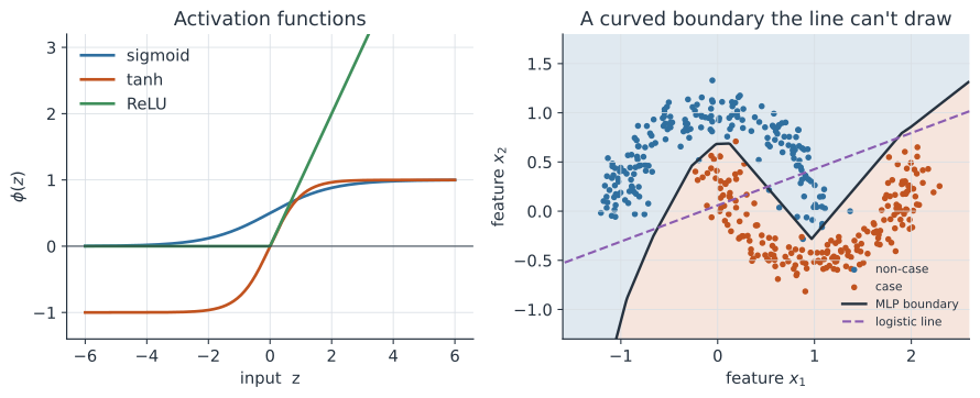
The nonlinearity is essential. Compose two linear layers and you get $W_2(W_1\mathbf{x}) = (W_2 W_1)\mathbf{x}$, still linear — no depth is bought. The activation $\phi$ between layers is what lets the network bend, so a two-layer MLP can carve the curved boundary in the figure that no single line can.

Activation functions#

Three activations cover most practice, shown on the left of the figure. The sigmoid $\phi(z) = 1/(1+e^{-z})$ squashes to $(0,1)$ and is the natural choice for a probability output. The hyperbolic tangent $\tanh(z)$ squashes to $(-1,1)$ and is zero-centred, which helps hidden layers. The rectified linear unit $\mathrm{ReLU}(z) = \max(0, z)$ is the modern default for hidden layers: it is cheap, and because its slope is exactly $1$ for positive inputs it does not “saturate” and choke off gradients the way the sigmoid does deep in a network.

Why depth expresses so much#

The universal approximation theorem says an MLP with a single hidden layer and enough units can approximate any continuous function on a bounded domain to arbitrary accuracy. Depth makes this efficient: composing layers builds features hierarchically, so early layers detect simple structure and later layers combine it into complex concepts, often with far fewer total units than a single wide layer would need. This is the same feature-building logic that convolutional networks exploit for images and that recurrent networks exploit for sequences.

Training: loss, gradients, and backpropagation#

The network’s weights start random and are learned by minimizing a loss that measures prediction error. For binary classification the loss is the same binary cross-entropy used in logistic regression, $$\mathcal{L} = -\frac{1}{n}\sum_{i=1}^{n} \Bigl[ y_i \log \hat{p}_i + (1-y_i)\log(1-\hat{p}_i) \Bigr],$$ where $\hat{p}_i$ is the network’s output probability for example $i$; for regression it is mean squared error. We minimize $\mathcal{L}$ by gradient descent: repeatedly nudge every weight a small step $\eta$ (the learning rate) down its gradient, $$W^{(l)} \leftarrow W^{(l)} - \eta\, \frac{\partial \mathcal{L}}{\partial W^{(l)}}.$$

The efficient way to get every partial derivative at once is backpropagation — the chain rule applied layer by layer, from the output back to the input. Define the error signal at layer $l$ as $\boldsymbol{\delta}^{(l)} = \partial \mathcal{L}/\partial \mathbf{z}^{(l)}$. It starts at the output as $\hat{\mathbf{p}} - \mathbf{y}$ and propagates backward through $$\boldsymbol{\delta}^{(l)} = \left(W^{(l+1)\top}\boldsymbol{\delta}^{(l+1)}\right) \odot \phi'\!\left(\mathbf{z}^{(l)}\right),$$ where $\odot$ is the elementwise product and $\phi'$ the activation’s derivative. Each layer’s weight gradient is then the outer product $\partial\mathcal{L}/\partial W^{(l)} = \boldsymbol{\delta}^{(l)} \mathbf{a}^{(l-1)\top}$. In practice the gradient is averaged over a small random mini-batch of examples rather than the whole dataset each step — stochastic gradient descent — which is cheaper and adds helpful noise; optimizers such as Adam adapt the step size per weight on top of this.

A worked example#

Take one hidden neuron with weights $\mathbf{w}_1 = (1, -1)$, bias $b_1 = 0$, ReLU activation, feeding an output neuron with weight $w_2 = 2$, bias $b_2 = -0.5$, sigmoid activation. For the input $\mathbf{x} = (2, 1)$ the hidden pre-activation is $z_1 = 1\cdot 2 + (-1)\cdot 1 + 0 = 1$, so $a_1 = \mathrm{ReLU}(1) = 1$. The output pre-activation is $z_2 = 2\cdot 1 - 0.5 = 1.5$, giving $\hat{p} = 1/(1+e^{-1.5}) = 0.818$. If the true label is $y = 1$, the output error is $\hat{p} - y = -0.182$, which backpropagation pushes through $w_2$ and the ReLU (slope $1$ here) to update both neurons’ weights so the next forward pass on this example returns a probability a little closer to $1$.

In code#

Python#

A multilayer perceptron is short enough to write from scratch — one forward pass, one backprop, and a gradient step — which is the best way to see that there is no magic inside.

import numpy as np
rng = np.random.default_rng(0)

# toy nonlinear task: "case" vs "non-case" in two features (interleaving moons)
n = 200
t = rng.uniform(0, np.pi, n)
Xa = np.c_[np.cos(t), np.sin(t)] + 0.12 * rng.standard_normal((n, 2))
Xb = np.c_[1 - np.cos(t), 0.5 - np.sin(t)] + 0.12 * rng.standard_normal((n, 2))
X = np.vstack([Xa, Xb])
y = np.r_[np.zeros(n), np.ones(n)][:, None]

W1 = 0.5 * rng.standard_normal((2, 16)); b1 = np.zeros(16)   # 2 -> 16 hidden
W2 = 0.5 * rng.standard_normal((16, 1)); b2 = np.zeros(1)    # 16 -> 1 output
lr = 1.0
for epoch in range(5001):
    h = np.maximum(0, X @ W1 + b1)                 # ReLU hidden activations
    p = 1 / (1 + np.exp(-(h @ W2 + b2)))           # sigmoid output probability
    dout = (p - y) / len(X)                         # output error signal
    dh = (dout @ W2.T) * (h > 0)                    # backprop through ReLU
    W2 -= lr * h.T @ dout; b2 -= lr * dout.sum(0)   # gradient step
    W1 -= lr * X.T @ dh;   b1 -= lr * dh.sum(0)
    if epoch % 1000 == 0:
        loss = -np.mean(y * np.log(p + 1e-9) + (1 - y) * np.log(1 - p + 1e-9))
        print(f"epoch {epoch:4d}  loss {loss:.3f}")
print(f"train accuracy {np.mean((p > 0.5) == y):.3f}")

epoch    0  loss 0.847
epoch 1000  loss 0.039
epoch 2000  loss 0.028
epoch 3000  loss 0.025
epoch 4000  loss 0.024
epoch 5000  loss 0.023
train accuracy 0.988

In real work you would not hand-roll this; a framework builds the same network, computes the gradients automatically, and runs on a GPU. The idiomatic version builds the same network in PyTorch, which computes the gradients automatically and runs on a GPU when one is present — the same 2→16→1 model, trained on the moons data from above:

import torch, torch.nn as nn
torch.manual_seed(0)

model = nn.Sequential(nn.Linear(2, 16), nn.ReLU(), nn.Linear(16, 1))
opt = torch.optim.Adam(model.parameters(), lr=1e-2)
Xt, yt = torch.tensor(X, dtype=torch.float32), torch.tensor(y, dtype=torch.float32)

for epoch in range(2000):
    opt.zero_grad()
    loss = nn.functional.binary_cross_entropy_with_logits(model(Xt), yt)
    loss.backward()        # autograd does the backprop for you
    opt.step()
acc = ((model(Xt) > 0).float() == yt).float().mean().item()
print(f"parameters: {sum(p.numel() for p in model.parameters())}")
print(f"train accuracy: {acc:.2f}")

parameters: 65
train accuracy: 1.00

For a quick, dependable classifier without writing any network code, scikit-learn’s MLPClassifier fits the same architecture with one call:

from sklearn.neural_network import MLPClassifier
clf = MLPClassifier(hidden_layer_sizes=(16, 16), max_iter=2000,
                    random_state=0).fit(X, y.ravel())
print(f"sklearn MLP accuracy {clf.score(X, y.ravel()):.3f}")

sklearn MLP accuracy 0.983

R#

# nnet fits a single-hidden-layer network; torch/keras for deeper models.
library(nnet)
set.seed(1)
df <- data.frame(x1 = X[, 1], x2 = X[, 2], y = factor(y))
fit <- nnet(y ~ x1 + x2, data = df, size = 16, maxit = 500, trace = FALSE)
mean(predict(fit, df, type = "class") == df$y)   # training accuracy

Julia#

# Flux builds and trains networks with automatic differentiation.
using Flux
model = Chain(Dense(2 => 16, relu), Dense(16 => 1), sigmoid)
loss(m, x, y) = Flux.binarycrossentropy(m(x), y)
opt = Flux.setup(Adam(0.01), model)
for epoch in 1:2000
    Flux.train!(loss, model, [(X', y')], opt)
end

Why it matters#

Neural networks are the substrate under most of modern applied machine learning, and the epidemiological uses follow directly from the pieces above. An MLP is a flexible nonlinear classifier or regressor: predict severe outcomes from a patient’s covariates, or a nowcast from a bundle of surveillance signals, when the relationships are too curved for a GLM. Swap the architecture and the same training machinery specializes — recurrent networks for case-count time series, convolutional networks for medical images, and variational autoencoders for representation learning and anomaly detection. The caution is the same everywhere: a network’s flexibility makes it easy to overfit and hard to interpret, so honest validation on held-out data, calibration checks, and awareness of the training data’s biases matter more here than with a transparent regression, not less.

Related#

• Logistic Regression
• Generalized Linear Models
• The Chain Rule
• The Gradient
• Optimization and Critical Points
• Recurrent Networks and LSTMs
• Variational Autoencoders
• Convolutional Networks and Image Identification
• Deep Learning, Foundation Models, and Agentic AI
• Quantitative Methods