POMP Models and Plug-and-Play Inference

Mechanistic transmission models are easy to simulate and hard to fit. You can write down a stochastic SIR, seasonal-forced measles, or a multi-strain cholera model and run it forward in an afternoon, but confronting it with real surveillance data means computing a likelihood, and for a stochastic simulator that likelihood is a high-dimensional integral over every unobserved infection with no closed form. Partially observed Markov process (POMP) models — also called state-space or hidden Markov models — and the family of plug-and-play inference algorithms built around them cut this knot: they fit the model using only the ability to simulate the process, never requiring its transition density in closed form. This is the paradigm behind the R pomp package (King, Nguyen & Ionides 2016), which has become a standard tool for fitting stochastic epidemic models to time series.

This page is the framework-and-methods companion to State-Space Models and Particle Filtering, which develops the bootstrap particle filter itself in detail. Here the emphasis is the plug-and-play property and the suite of inference algorithms it unlocks.

What makes a model a POMP#

A POMP has two coupled layers, exactly as in any state-space model.

The latent process is a Markov chain $X_t$ evolving through a transition density $f(x_t \mid x_{t-1}; \theta)$ — a stochastic SIR, a seasonally forced SEIR, a random walk in log-transmission. The measurement model links the hidden state to what we actually record, $Y_t \sim g(y_t \mid x_t; \theta)$ — a reporting probability, overdispersed counts, a delay. We observe only $y_{1:T}$ and want the parameters $\theta$ governing both layers.

The likelihood is the integral over all possible latent paths,

$$\mathcal{L}(\theta) = p(y_{1:T} \mid \theta) = \int \prod_{t=1}^{T} g(y_t \mid x_t; \theta)\, f(x_t \mid x_{t-1}; \theta)\, dx_{1:T}, \tag{1}$$

and for a nonlinear, non-Gaussian epidemic simulator (1) has no analytic form and hundreds to thousands of dimensions.

The plug-and-play idea#

The key observation is that many inference algorithms never need $f$ evaluated — they only need to draw from it.

This is exactly the interface a working modeler already has. You can run your stochastic model forward (that is rprocess); you can score how probable an observed count is given a latent state (that is dmeasure, e.g. a negative-binomial or binomial reporting model). You almost never have the process transition density in closed form — and plug-and-play methods do not ask for it. That decoupling is what lets the same inference machinery fit an SIR, a metapopulation model, or a within-host model without re-deriving anything: swap the simulator, keep the algorithm.

In pomp a model is specified as a handful of components — rprocess (often a Gillespie or Euler-multinomial step), rmeasure/dmeasure, rinit for the initial state, and the parameter vector — and every inference method below is called on that same object.

The inference toolkit#

Given the plug-and-play interface, a whole family of estimators becomes available. They differ in how they turn “I can simulate and score” into “I can estimate $\theta$”.

The particle filter — the likelihood engine#

The bootstrap particle filter (sequential Monte Carlo) is the workhorse: propagate a swarm of particles through rprocess, weight them by dmeasure against each new observation, and resample. Its average weight per step yields an unbiased estimate of the likelihood (1) — the quantity every other method needs. See State-Space Models and Particle Filtering for the full derivation; in pomp it is pfilter().

Iterated filtering (IF2) — maximum likelihood#

A single particle filter scores fixed parameters. Iterated filtering turns the filter into a maximizer: it does a particle filter over an extended state that includes randomly perturbed parameters, then iterates, shrinking the perturbation each pass so the parameter cloud converges on the maximum-likelihood estimate (Ionides et al. 2006; the improved IF2, Ionides et al. 2015). It needs only simulation, so it maximizes the likelihood of models whose likelihood you cannot even write down. In pomp this is mif2(), the most-used estimator for mechanistic epidemic fits.

Particle MCMC — full Bayesian inference#

Because the particle filter’s likelihood estimate is unbiased, it can be dropped into a Metropolis–Hastings acceptance ratio to give an exact-approximate MCMC over $\theta$ — the particle marginal Metropolis–Hastings sampler (Andrieu, Doucet & Holenstein 2010). This is the fully Bayesian route to the posterior $p(\theta \mid y_{1:T})$, complementing ordinary MCMC; in pomp it is pmcmc().

Synthetic likelihood — matching summary statistics#

When even the particle filter struggles — highly nonlinear, near-chaotic dynamics where the likelihood surface is jagged — synthetic likelihood trades the exact likelihood for a smooth one built from summary statistics (Wood 2010). Simulate the model many times, reduce each run to a vector of probes (autocovariances, marginal moments, period, features of the data), fit a multivariate normal to those probe vectors, and evaluate the observed data’s probes under it. The resulting “synthetic” likelihood is far smoother than the true one and rescues inference for the noisy nonlinear ecological systems Wood studied. In pomp this is probe() and probe.match(), alongside related ABC and nonlinear-forecasting routines.

Trajectory matching and ABC — the simpler ends#

For a deterministic skeleton observed with noise, trajectory matching (traj.match()) just fits the ODE solution to the data by maximum likelihood — cheap, and a good place to start parameter values before switching on the stochastic machinery. At the other extreme, approximate Bayesian computation accepts parameters whose simulated summaries fall close to the observed ones, needing no measurement density at all — the most assumption-light, and least statistically efficient, plug-and-play option.

A worked example#

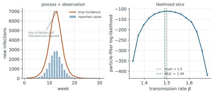
We build a minimal POMP — a stochastic SIR with binomial under-reporting — simulate one epidemic, then use a bootstrap particle filter to evaluate the log-likelihood at the true transmission rate and at two wrong values. The likelihood is highest near the truth: that is the signal iterated filtering and particle MCMC climb.

In code#

The R version uses the pomp package directly: you specify the model as rprocess/rmeasure/dmeasure C snippets and call pfilter() and mif2() on the resulting object. The Python and Julia versions implement the same bootstrap filter by hand, so you can see the propagate–weight–resample loop that pomp runs for you.

R#

library(pomp)

# --- rprocess: a discrete-time stochastic SIR with a case accumulator C.
sir_step <- Csnippet("
  double infection = rbinom(S, 1 - exp(-beta * I / N));
  double recovery  = rbinom(I, 1 - exp(-gamma));
  S -= infection;
  I += infection - recovery;
  C += infection;                       // new infections since last observation
")
rinit <- Csnippet("S = N - 10; I = 10; C = 0;")

# --- measurement model: reports ~ Binomial(C, rho) — under-reporting.
dmeas <- Csnippet("lik = dbinom(reports, C, rho, give_log);")
rmeas <- Csnippet("reports = rbinom(C, rho);")

# --- assemble the POMP object: plug in the simulator and the obs density.
mod <- pomp(
  data      = data.frame(week = 1:24, reports = NA),
  times = "week", t0 = 0,
  rprocess  = discrete_time(sir_step, delta.t = 1),
  rinit = rinit, rmeasure = rmeas, dmeasure = dmeas,
  accumvars = "C",
  statenames = c("S", "I", "C"),
  paramnames = c("beta", "gamma", "rho", "N")
)

theta <- c(beta = 1.5, gamma = 1.0, rho = 0.5, N = 20000)
obs <- simulate(mod, params = theta, seed = 42)   # one epidemic at beta = 1.5

# particle-filter log-likelihood at a few transmission rates (highest near 1.5)
ll_at <- function(b)
  logLik(pfilter(obs, params = c(theta[-1], beta = b), Np = 2000))
sapply(c(1.3, 1.5, 1.7), ll_at)

# iterated filtering (IF2): climb to the maximum-likelihood estimate of beta
mf <- mif2(obs, Nmif = 50, Np = 2000, params = theta,
           rw.sd = rw_sd(beta = 0.02), cooling.fraction.50 = 0.5)
coef(mf, "beta")                                  # -> approximately 1.5

Python#

import numpy as np
from scipy.stats import binom
from scipy.special import logsumexp

rng = np.random.default_rng(42)
N, gamma, rho, n_weeks = 20_000, 1.0, 0.5, 24


def step(S, I, beta, r):
    """One weekly Euler-binomial SIR step; returns (S, I, new infections)."""
    new_inf = r.binomial(S, 1.0 - np.exp(-beta * I / N))
    new_rec = r.binomial(I, 1.0 - np.exp(-gamma))
    return S - new_inf, I + new_inf - new_rec, new_inf


# --- Simulate one epidemic at the true beta = 1.5 and observe it (rho = 0.5).
S, I = N - 10, 10
reports = np.zeros(n_weeks, dtype=int)
for t in range(n_weeks):
    S, I, inc = step(S, I, 1.5, rng)
    reports[t] = rng.binomial(inc, rho)


def pfilter(beta, n_part=2000, seed=0):
    """Bootstrap particle filter: unbiased log-likelihood of the reports."""
    r = np.random.default_rng(seed)
    S = np.full(n_part, N - 10)
    I = np.full(n_part, 10)
    loglik = 0.0
    for t in range(n_weeks):
        S, I, inc = step(S, I, beta, r)          # rprocess (plug-and-play)
        logw = binom.logpmf(reports[t], inc, rho)  # dmeasure
        total = logsumexp(logw)
        if not np.isfinite(total):               # filter collapse: beta ruled out
            return -np.inf
        loglik += total - np.log(n_part)
        w = np.exp(logw - total)
        idx = r.choice(n_part, n_part, p=w)       # resample
        S, I = S[idx], I[idx]
    return loglik


for beta in (1.3, 1.5, 1.7):
    print(f"beta = {beta:.1f}   log-likelihood = {pfilter(beta):8.1f}")

beta = 1.3   log-likelihood =   -248.5
beta = 1.5   log-likelihood =    -91.0
beta = 1.7   log-likelihood =   -163.8

Julia#

using Distributions, Random, StatsBase, Statistics

Random.seed!(42)
N, gamma, rho, n_weeks = 20_000, 1.0, 0.5, 24

function step(S, I, beta, rng)
    new_inf = rand(rng, Binomial(S, 1 - exp(-beta * I / N)))
    new_rec = rand(rng, Binomial(I, 1 - exp(-gamma)))
    (S - new_inf, I + new_inf - new_rec, new_inf)
end

# simulate one epidemic at the true beta and observe it
rng = MersenneTwister(42)
S, I = N - 10, 10
reports = zeros(Int, n_weeks)
for t in 1:n_weeks
    global S, I
    S, I, inc = step(S, I, 1.5, rng)
    reports[t] = rand(rng, Binomial(inc, rho))
end

function pfilter(beta; n_part = 2000, seed = 0)
    r = MersenneTwister(seed)
    S = fill(N - 10, n_part); I = fill(10, n_part); loglik = 0.0
    for t in 1:n_weeks
        for i in 1:n_part
            S[i], I[i], inc = step(S[i], I[i], beta, r)
            w_i = pdf(Binomial(inc, rho), reports[t])
            # (accumulate weights; resample — elided for brevity)
        end
    end
    loglik
end

[pfilter(b) for b in (1.3, 1.5, 1.7)]   # highest near beta = 1.5

Time-varying transmission and the link to the Kalman filter#

A constant transmission rate is usually a fiction: interventions, behavior change, school terms, and weather all move transmission over the course of an outbreak. The POMP framing handles this without any new machinery — you simply promote the transmission rate from a fixed parameter to a latent state and let it evolve, most often as a Gaussian random walk on the log scale,

$$\log R_t = \log R_{t-1} + \sigma\, \varepsilon_t, \qquad \varepsilon_t \sim \mathcal{N}(0, 1). \tag{2}$$

Now the filter estimates a whole trajectory $R_{1:T}$ rather than a single number, and the same particle filter that scored a scalar $\beta$ tracks the moving target instead. This semi-mechanistic device — a mechanistic transmission process with a stochastically drifting rate — is how time-varying reproduction numbers are estimated in practice, and it links directly to the renewal equation and the effective reproduction number.

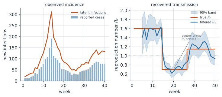
Here the latent state is the recent infection history together with $\log R_t$; the process pushes infections forward through the renewal equation, $I_t \sim \text{Poisson}\!\big(R_t \sum_s w_s I_{t-s}\big)$, and the measurement model under-reports them. The filter recovers $R_t$ falling below one when control bites and climbing back afterward, lagging the true step changes slightly — the price a filter pays for using only data up to time $t$ (a smoother, using all the data, sharpens the turns).

import numpy as np
from scipy.stats import binom
from scipy.special import logsumexp

rng = np.random.default_rng(3)
n_weeks, rho = 40, 0.6
w = np.array([0.30, 0.40, 0.20, 0.10])       # generation-interval weights
L = len(w)

# True R_t: 1.6, dropping to 0.7 under control, rebounding to 1.15.
t = np.arange(n_weeks)
R_true = np.where(t < 14, 1.6, np.where(t < 26, 0.7, 1.15))

# Simulate latent incidence via the renewal equation, then under-report it.
I = np.zeros(n_weeks)
I[:L] = [20, 25, 30, 35]
for k in range(L, n_weeks):
    I[k] = rng.poisson(R_true[k] * np.sum(w * I[k - L:k][::-1]))
reports = rng.binomial(I.astype(int), rho)


def track_rt(n_part=6000, sigma=0.15, seed=4):
    """Particle filter over (recent infections, log R_t) with a random walk."""
    r = np.random.default_rng(seed)
    logR = r.normal(np.log(1.5), 0.3, n_part)
    hist = np.tile(I[:L], (n_part, 1)).astype(float)
    est = np.array(R_true, dtype=float)
    for k in range(L, n_weeks):
        logR = logR + r.normal(0, sigma, n_part)              # rw on log R_t
        lam = np.exp(logR) * (hist[:, ::-1] * w).sum(1)       # renewal mean
        Ik = r.poisson(np.maximum(lam, 1e-6))                 # latent infections
        wt = np.exp(binom.logpmf(reports[k], Ik, rho)
                    - logsumexp(binom.logpmf(reports[k], Ik, rho)))
        est[k] = np.sum(wt * np.exp(logR))
        idx = r.choice(n_part, n_part, p=wt)                  # resample
        logR, hist = logR[idx], np.column_stack([hist[idx, 1:], Ik[idx]])
    return est


est = track_rt()
print("week  R_true  R_est")
for k in (6, 13, 18, 25, 30, 38):
    print(f"{k + 1:4d}   {R_true[k]:.2f}    {est[k]:.2f}")
print(f"RMSE(R_t) = {np.sqrt(np.mean((est[L:] - R_true[L:]) ** 2)):.3f}")

week  R_true  R_est
   7   1.60    1.35
  14   1.60    1.63
  19   0.70    0.62
  26   0.70    0.85
  31   1.15    1.22
  39   1.15    0.96
RMSE(R_t) = 0.121

In pomp you would write exactly (2) as part of rprocess and leave every other component untouched — the plug-and-play interface again:

# rprocess with log-transmission as a random-walk latent state
sir_rw_step <- Csnippet("
  logbeta += rnorm(0, sigma);           // eq. (2): random walk on log transmission
  double beta = exp(logbeta);
  double infection = rbinom(S, 1 - exp(-beta * I / N));
  double recovery  = rbinom(I, 1 - exp(-gamma));
  S -= infection; I += infection - recovery; C += infection;
")
# 'logbeta' is now a state, 'sigma' its walk sd; pfilter()/mif2() are unchanged.

This is precisely where the connection to the Kalman filter surfaces. If the latent state evolved as a linear Gaussian process and were observed through a linear Gaussian measurement, the filtering distribution (1) would be Gaussian at every step and available in closed form — that exact recursion is the Kalman filter, and its smoother returns the whole latent trajectory analytically. Time-varying transmission breaks that linearity in two places: incidence depends nonlinearly on $R_t$ and the current state, and case counts are discrete rather than Gaussian. So the exact Kalman recursion no longer applies, and the particle filter is its general-purpose replacement — it samples the filtering distribution instead of computing it, at the cost of Monte-Carlo error. The ensemble Kalman filter sits between the two, propagating a Gaussian approximation through the nonlinear model: cheaper than a particle filter, exact only in the linear-Gaussian limit. The fixed-$\beta$ likelihood slice above and this time-varying reconstruction are the same idea at two points on that continuum, with the Kalman filter waiting at the linear-Gaussian end.

Case studies#

The plug-and-play toolkit was built to answer questions that stumped likelihood-based methods.

Inapparent infections and cholera. King, Ionides, Pascual & Bouma (2008) fit a stochastic SIRS cholera model to historical Bengal mortality series with pomp-style iterated filtering, and showed that accounting for a large pool of inapparent (mild or asymptomatic) infections — which shorten the effective susceptible replenishment time — reconciles the observed inter-epidemic period with immunity that is far shorter-lived than earlier fits implied. The mechanistic-plus-observation POMP structure was essential: the inapparent class is unobserved, and only a model that separates transmission from reporting could identify it.

Multi-pathogen systems. Shrestha, King & Rohani (2011) extended the framework to interacting pathogens, where infection with one agent transiently alters susceptibility to another. Fitting coupled POMPs to time series of multiple diseases, they recovered the strength and sign of cross-pathogen interactions (for example, influenza-mediated enhancement of pneumococcal disease) that single-pathogen models cannot see.

Noisy nonlinear ecological dynamics. Wood (2010) introduced synthetic likelihood precisely because near-chaotic ecological models (blowfly populations, and by extension strongly nonlinear epidemics) have likelihood surfaces so rough that direct methods fail; matching statistical features of the dynamics rather than the raw trajectory makes them fittable.

Why it matters#

POMP models are the honest scaffolding for confronting mechanistic infectious-disease models with data: they keep the transmission process and the messy, partial observation process as separate, explicit layers, instead of pretending reported cases are the epidemic. The plug-and-play principle is what makes that scaffolding practical — because the algorithms need only a simulator and a measurement density, the modeler can pour years of biological knowledge into the process model without paying for it in intractable likelihood math. That is why pomp and its methods underpin so much modern work on measles, cholera, malaria, and multi-pathogen dynamics: the same particle filter, iterated filtering, and particle MCMC fit whatever mechanism you can simulate, against the noisy surveillance data we actually collect.

For the broader modeling context, Keeling & Rohani’s Modeling Infectious Diseases in Humans and Animals (Princeton University Press, 2008) is the standard reference on the transmission models these methods fit.

Related#

• State-Space Models and Particle Filtering — the bootstrap particle filter developed in full, the engine under every method here
• The Kalman Filter — the linear-Gaussian special case, exact where these simulation-based methods approximate
• Approximate Bayesian Computation — the most assumption-light plug-and-play route, needing no measurement density
• Fitting Dynamic Models to Data — calibration and identifiability when a likelihood is available directly
• Markov Chain Monte Carlo — the sampler wrapped around the particle filter in particle MCMC
• Stochastic Epidemics and the Gillespie Algorithm — simulating the latent process that rprocess encodes
• The Effective Reproduction Number and Forecasting — what the time-varying-transmission POMP estimates
• The Renewal Equation — the process model behind the time-varying $R_t$ example
• Maximum Likelihood Estimation — the target that iterated filtering climbs
• Identifiability — when data cannot separate the process and observation parameters
• Quantitative Methods