Phylogenetic Inference: Substitution Models and Tree Building
A phylogenetic tree is not observed; it is estimated from sequences, and every downstream method — the molecular clock, the coalescent, phylodynamics, transmission-tree reconstruction — takes that tree as input. Getting it right means a model of how sequences change over time, a way to score any candidate tree against the data, and a search through the vast space of possible trees. This page walks through the pieces and ends by running the standard tools on data we simulate ourselves.
Substitution models#
The engine of phylogenetics is a continuous-time Markov model of how one nucleotide turns into another. It is defined by a rate matrix whose off-diagonal entries are instantaneous substitution rates, and the probability of change over a branch of length (measured in expected substitutions per site) is the matrix exponential
Models form a nested hierarchy of increasing realism. JC69 (Jukes-Cantor) assumes all substitutions are equally likely and all bases equally frequent. K80 adds a transition/transversion bias, HKY adds unequal base frequencies, and GTR (general time-reversible) allows a distinct rate for each pair of bases — the most general reversible model. Two add-ons matter in practice: +G lets the substitution rate vary across sites by a gamma distribution (most sites evolve slowly, a few fast), and +I allows a fraction of invariant sites. Choosing among them is model selection, done automatically by tools like ModelFinder.
For the simplest model, JC69, has a closed form: the probability a site is unchanged is , and the probability of any particular change is .
import numpy as np

# JC69 transition probabilities over a branch of length t (subs/site).
def p_same(t):
    return 0.25 + 0.75 * np.exp(-4 / 3 * t)

def p_diff(t):
    return 0.25 - 0.25 * np.exp(-4 / 3 * t)

for t in [0.05, 0.2, 0.5, 1.0, 3.0]:
    print(f"t={t:<4}  P(no change)={p_same(t):.3f}  "
          f"P(a specific change)={p_diff(t):.3f}")
t=0.05  P(no change)=0.952  P(a specific change)=0.016
t=0.2   P(no change)=0.824  P(a specific change)=0.059
t=0.5   P(no change)=0.635  P(a specific change)=0.122
t=1.0   P(no change)=0.448  P(a specific change)=0.184
t=3.0   P(no change)=0.264  P(a specific change)=0.245
Distances and the saturation problem#
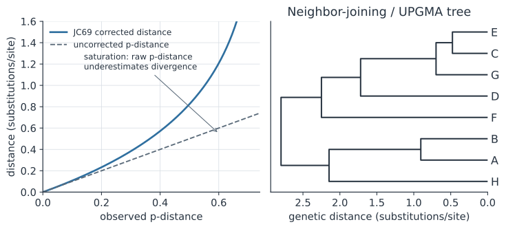
The quickest way to a tree is through pairwise distances. The raw p-distance — the fraction of sites at which two sequences differ — underestimates true divergence, because as time passes some sites mutate more than once and a few even mutate back, so observed differences saturate while real substitutions keep accumulating. The substitution model supplies the correction; for JC69 it is
which is the curve in the left panel of the figure, diverging from the raw p-distance and blowing up as .
def jc69_distance(p):
    """Jukes-Cantor genetic distance from the observed p-distance."""
    return -0.75 * np.log(1 - (4 / 3) * p)

for p in [0.05, 0.15, 0.30, 0.45, 0.60]:
    print(f"p-distance {p:.2f}  ->  JC69 distance {jc69_distance(p):.3f}")
p-distance 0.05  ->  JC69 distance 0.052
p-distance 0.15  ->  JC69 distance 0.167
p-distance 0.30  ->  JC69 distance 0.383
p-distance 0.45  ->  JC69 distance 0.687
p-distance 0.60  ->  JC69 distance 1.207
Given a matrix of corrected distances, neighbor-joining builds a tree by repeatedly joining the pair of taxa that minimizes total branch length, and it is fast enough for thousands of sequences, which is why it is the standard first pass and the starting tree for likelihood methods.
Scoring a tree: the pruning algorithm#
Distances throw away information; maximum likelihood and Bayesian methods use the full alignment by computing the probability of the data given a tree, its branch lengths, and the substitution model. The key that makes this tractable is Felsenstein’s pruning algorithm, which computes the likelihood of a site by working from the tips to the root, carrying at each node a vector of conditional likelihoods — the probability of the observed tip data below that node, given each possible nucleotide at the node (Felsenstein 1981). Here it is for a single site on a small rooted tree.
def P_jc(t):
    """JC69 4x4 transition-probability matrix for branch length t."""
    e = np.exp(-4 / 3 * t)
    P = np.full((4, 4), 0.25 - 0.25 * e)
    np.fill_diagonal(P, 0.25 + 0.75 * e)
    return P

def tip(base):                      # A=0, C=1, G=2, T=3
    v = np.zeros(4); v[base] = 1.0
    return v

def down(child_L, t):               # contribution of a child branch
    return P_jc(t) @ child_L

# Tree ((A,B),(C,D)); observed bases at this site: A=A, B=A, C=C, D=G.
LX = down(tip(0), 0.05) * down(tip(0), 0.06)     # internal node above A, B
LY = down(tip(1), 0.05) * down(tip(2), 0.07)     # internal node above C, D
Lroot = down(LX, 0.10) * down(LY, 0.10)          # root
site_lik = 0.25 * Lroot.sum()                    # equal base frequencies

print(f"site likelihood      = {site_lik:.3e}")
print(f"site log-likelihood  = {np.log(site_lik):.3f}")
site likelihood      = 5.493e-04
site log-likelihood  = -7.507
The likelihood of the whole alignment is the product over sites, and searching tree space — rearranging branches by nearest-neighbor interchange or subtree pruning and regrafting — finds the tree that maximizes it. Because that space is astronomically large, the search is heuristic, and bootstrap resampling of alignment columns quantifies how well-supported each branch is. Bayesian inference instead samples trees in proportion to their posterior probability with MCMC, returning a distribution over trees and, when tips are dated, a time-scaled tree with a molecular clock.
Generating data to try it#
To make the tools concrete, we simulate an alignment by evolving sequences down a known tree under JC69, then reconstruct with neighbor-joining and print the tree.
rng = np.random.default_rng(1834)
L = 800

def evolve(seq, t):
    """Evolve a sequence along a branch of length t under JC69."""
    p_change = 0.75 * (1 - np.exp(-4 / 3 * t))
    change = rng.random(seq.size) < p_change
    out = seq.copy()
    out[change] = (seq[change] + rng.integers(1, 4, change.sum())) % 4
    return out

anc = rng.integers(0, 4, L)                 # random ancestral sequence
nAB, nCD, nEF = evolve(anc, 0.10), evolve(anc, 0.12), evolve(anc, 0.15)
seqs = {"A": evolve(nAB, 0.05), "B": evolve(nAB, 0.06),
        "C": evolve(nCD, 0.05), "D": evolve(nCD, 0.07),
        "E": evolve(nEF, 0.08), "F": evolve(nEF, 0.06)}

# JC-corrected pairwise distance matrix.
names = list(seqs)
arr = np.array([seqs[n] for n in names])
D = np.array([[jc69_distance(np.mean(arr[a] != arr[b]))
               for b in range(len(names))] for a in range(len(names))])

def neighbor_joining(labels, D):
    labels, D = list(labels), D.astype(float).copy()
    while len(labels) > 2:
        n = len(labels)
        r = D.sum(1)
        Q = (n - 2) * D - r[:, None] - r[None, :]
        np.fill_diagonal(Q, np.inf)
        i, j = np.unravel_index(np.argmin(Q), Q.shape)
        di = 0.5 * D[i, j] + (r[i] - r[j]) / (2 * (n - 2))
        node = f"({labels[i]}:{di:.3f},{labels[j]}:{D[i, j] - di:.3f})"
        new = 0.5 * (D[i] + D[j] - D[i, j])
        keep = [k for k in range(n) if k not in (i, j)]
        D = np.vstack([np.column_stack([D[np.ix_(keep, keep)], new[keep]]),
                       np.append(new[keep], 0.0)])
        labels = [labels[k] for k in keep] + [node]
    return f"({labels[0]}:{D[0, 1] / 2:.3f},{labels[1]}:{D[0, 1] / 2:.3f});"

print("neighbor-joining tree (Newick):")
print(neighbor_joining(names, D))
neighbor-joining tree (Newick):
((A:0.026,B:0.050):0.052,((E:0.081,F:0.050):0.155,(C:0.052,D:0.087):0.113):0.052);
The reconstruction recovers the three simulated pairs — (A,B), (C,D), (E,F) — as clades, which is the tree we evolved down.
Maximum likelihood with IQ-TREE#
For real analysis you would write those sequences to alignment.fasta and hand them to a dedicated program.
IQ-TREE finds the maximum-likelihood tree, selects the substitution model, and computes branch support in one command (Minh et al. 2020).
# ModelFinder picks the model; -B runs 1000 ultrafast bootstraps.
iqtree2 -s alignment.fasta -m MFP -B 1000 -T AUTO
-m MFPruns ModelFinder Plus, testing substitution models (JC, HKY, GTR, each with +G/+I) and choosing the best by BIC before inferring the tree.-B 1000gives 1000 ultrafast bootstrap replicates, so each branch carries a support percentage.- The results land in
alignment.fasta.treefile(the ML tree in Newick),alignment.fasta.iqtree(a report naming the selected model and its parameters), and.log.
Bayesian dating with BEAST#
When the sequences are time-stamped — sampled on known dates — BEAST infers a dated tree and a substitution rate jointly, sampling the posterior over trees with MCMC (Bouckaert et al. 2019). The workflow is a short pipeline of programs.
1. BEAUti  — load alignment.fasta, set the site model (e.g. HKY+G or GTR+G),
             the clock model (strict or relaxed molecular clock), and the tree
             prior (coalescent constant/exponential, or birth-death). Enter the
             tip dates. Save the analysis as beast.xml.
2. BEAST   — run the MCMC chain:
             beast -threads 4 beast.xml
3. Tracer  — check convergence: effective sample sizes (ESS) > 200 for the
             posterior, the clock rate, and the tree height.
4. TreeAnnotator — summarise the posterior tree sample into a maximum-clade-
             credibility tree with node dates and posterior support:
             treeannotator -burnin 10 beast.trees mcc.tree
5. FigTree / ggtree — visualise the dated tree with its credible intervals.
The payoff over IQ-TREE is a time tree with a credible interval on every node age and on the evolutionary rate, which is what feeds molecular-clock dating, phylodynamics, and the time-scaled phylogeny that TransPhylo turns into a transmission tree.
The same steps in R#
The ape and phangorn packages cover the distance and likelihood methods without leaving R.
library(ape); library(phangorn)

aln <- read.dna("alignment.fasta", format = "fasta")
D   <- dist.dna(aln, model = "JC69")     # JC-corrected distances
nj_tree <- nj(D)                          # neighbor-joining tree

phy <- as.phyDat(aln)                     # maximum likelihood with phangorn
fit <- pml(nj_tree, data = phy)
fit <- optim.pml(fit, model = "GTR", optGamma = TRUE)   # fit GTR+G
bs  <- bootstrap.pml(fit, bs = 100)       # bootstrap support
plotBS(fit$tree, bs)                       # ML tree with support values
Why it matters#
Every genomic-epidemiology result rests on a tree, and that tree carries the assumptions of a substitution model and the uncertainty of a heuristic search, so treating it as raw data hides both. Understanding the pieces — the rate matrix and , the distance correction that undoes saturation, the pruning likelihood that scores a tree, and the difference between an ML point estimate and a Bayesian posterior of dated trees — is what lets you choose a model, read a support value, and know when a clade is real. The tools do the heavy lifting; the judgment is yours.
Related#
- The Molecular Clock — turning a dated tree into rates and divergence times
- The Coalescent — the population-genetic model for the genealogy
- Phylodynamics — reading epidemic dynamics off the tree
- Detecting Selection with dN/dS — a substitution-rate ratio on coding sequences
- Transmission Tree Reconstruction — from a dated tree to who infected whom