Quasi-Stationary Distributions

Every closed stochastic epidemic ends the same way: sooner or later the last infectious individual recovers, transmission stops, and the process is stuck at zero forever. Extinction is the only true long-run state, so the honest stationary distribution of the chain puts all its mass on the disease-free state — a fact that says nothing about the years or centuries an endemic infection spends circulating first. The quasi-stationary distribution (QSD) is the object that describes that long transient: the prevalence a persistent infection hovers around conditioned on not having gone extinct yet.

The absorbing state that everything drifts toward#

Model the number infectious $I$ as a continuous-time Markov chain on the states $\{0, 1, 2, \dots, N\}$, exactly as in stochastic epidemics and the Gillespie algorithm. The state $I = 0$ is absorbing: with no infectious individuals and no external reintroduction, nothing in a closed population can create a new case, so once the chain hits zero it stays there. For any finite population the chain reaches zero with probability one, and the mathematically exact stationary distribution is the point mass $\delta_0$.

That limit is correct and useless. Measles circulated in large cities for generations, and endemic pathogens sit at a roughly stable prevalence for a very long time before any fade-out. To describe that behavior we condition on survival — we ask what the state looks like among the realizations that have not yet been absorbed — and the distribution that this conditioning settles into is the QSD.

Defining the quasi-stationary distribution#

Let $T = \inf\{t : I_t = 0\}$ be the extinction time, the first moment the chain is absorbed. A probability distribution $\nu = (\nu_1, \nu_2, \dots, \nu_N)$ over the transient states $\{1, \dots, N\}$ is quasi-stationary if starting the chain from $\nu$ leaves the survival-conditioned distribution unchanged for all time:

$$\Pr(I_t = j \mid I_0 \sim \nu,\ T > t) = \nu_j \qquad \text{for every } t \ge 0,\ j \ge 1. \tag{1}$$

It is the conditional analog of an ordinary stationary distribution: instead of $\nu$ being invariant under one step of the chain, it is invariant under one step of the chain restricted to the survivors. Just as an irreducible chain forgets its starting state and relaxes to its stationary distribution, a broad class of absorbing chains forgets where it started and relaxes to $\nu$ — the survival-conditioned distribution from any fixed start converges to the same QSD,

$$\lim_{t \to \infty} \Pr(I_t = j \mid T > t) = \nu_j, \tag{2}$$

a statement known as the Yaglom limit (Yaglom 1947; Darroch and Seneta 1967). Equation (2) is what makes the QSD a description of the endemic phase rather than an artifact of any particular seeding.

The eigenvalue picture#

The QSD is an eigenvector, in exact parallel with the stationary distribution being the left eigenvector $\pi = \pi P$ of a transition matrix. Write the generator of the continuous-time chain in block form, separating the absorbing state $0$ from the transient states $\{1, \dots, N\}$:

$$Q = \begin{pmatrix} 0 & \mathbf{0} \\ \mathbf{a} & C \end{pmatrix}.$$

Here $C$ is the sub-generator — the matrix of transition rates among the transient states — and $\mathbf{a}$ collects the rates of jumping from each transient state into extinction. Because probability leaks out of the transient block into the absorbing state, the rows of $C$ sum to something negative rather than zero, and all of its eigenvalues have negative real part. Let $-\lambda_1$ be the eigenvalue of $C$ with the largest real part (the one closest to zero), so $\lambda_1 > 0$ is the smallest decay rate. By a Perron–Frobenius argument for sub-stochastic matrices this leading eigenvalue is real and simple, and its left eigenvector — normalized to a probability vector — is the quasi-stationary distribution:

$$\nu\, C = -\lambda_1\, \nu, \qquad \sum_{j} \nu_j = 1,\ \ \nu_j \ge 0. \tag{3}$$

Every other mode of $C$ decays faster than $\lambda_1$, so after the fast transients die away the survivors are distributed according to $\nu$ and drain toward extinction through the single slow channel.

Extinction is an exponential clock#

The leading eigenvalue is not just a mathematical device; it is the extinction rate. Started from the QSD, the probability of still being alive decays exactly exponentially,

$$\Pr(T > t \mid I_0 \sim \nu) = e^{-\lambda_1 t}, \tag{4}$$

with no transient bends — the QSD is precisely the distribution that makes the fade-out hazard constant. The mean time to extinction from quasi-stationarity is therefore

$$\mathbb{E}[T \mid I_0 \sim \nu] = \frac{1}{\lambda_1}. \tag{5}$$

This is the single most useful number the QSD delivers: the expected persistence time of the endemic infection. Everything about whether a pathogen fades out or circulates indefinitely is encoded in how the slow eigenvalue $\lambda_1$ scales with population size and transmissibility.

A worked example: the stochastic SIS model#

The cleanest illustration is the stochastic SIS model, where recovered individuals return directly to susceptible so the whole state is captured by the number infectious $I$. In a population of size $N$ the two events and their rates are

• infection ($I \to I+1$) at rate $\displaystyle \beta\, \frac{I(N-I)}{N}$,
• recovery ($I \to I-1$) at rate $\gamma I$,

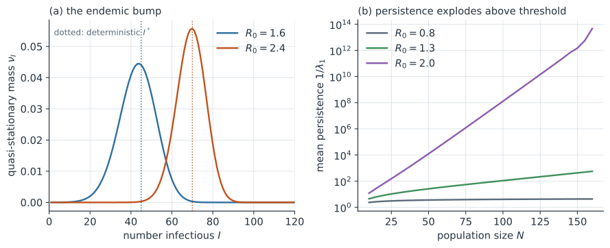
with $I = 0$ absorbing. Writing $R_0 = \beta/\gamma$, the deterministic SIS model has an endemic equilibrium at $I^\* = N(1 - 1/R_0)$ whenever $R_0 > 1$. The QSD is the stochastic counterpart of that fixed point: a bump concentrated around $I^\*$ with a roughly Gaussian shape and a width that grows like $\sqrt{N}$ (Figure 1, left panel). Where the deterministic model sits exactly at $I^\*$ forever, the stochastic model rattles around $I^\*$ in the shape of $\nu$ and, very occasionally, a run of bad luck walks it all the way down to zero.

The decisive fact is how the persistence time (5) scales. For $R_0 > 1$ the mean time to extinction grows exponentially in $N$: reaching zero requires the prevalence to fluctuate all the way from $I^\*$ down through every intermediate level against the restoring pull toward $I^\*$, and the probability of such a large deviation shrinks geometrically as the population grows (Nåsell 1996). For $R_0 < 1$ there is no endemic bump, the QSD piles up near $I = 1$, and extinction is quick. That contrast — slow, at most polynomial persistence below threshold versus exponential persistence above it — is the critical community size seen through the lens of a single eigenvalue.

In code#

We build the sub-generator $C$ for the stochastic SIS model, extract the quasi-stationary distribution as its leading left eigenvector, and read the persistence time straight off the eigenvalue. No simulation is needed — the QSD is exact linear algebra.

Python#

import numpy as np


def qsd(N, R0, gamma=1.0):
    """Quasi-stationary distribution nu and extinction rate lambda1
    for the stochastic SIS model on a population of size N."""
    beta = R0 * gamma
    I = np.arange(1, N + 1)                 # transient states 1..N
    up = beta * I * (N - I) / N             # infection rate
    down = gamma * I                        # recovery rate
    C = np.zeros((N, N))
    C[np.arange(N), np.arange(N)] = -(up + down)     # total outflow
    C[np.arange(N - 1), np.arange(1, N)] = up[:-1]   # I -> I+1
    C[np.arange(1, N), np.arange(N - 1)] = down[1:]  # I -> I-1
    vals, vecs = np.linalg.eig(C.T)         # left eigenvectors of C
    k = np.argmax(vals.real)               # eigenvalue closest to zero
    nu = np.abs(vecs[:, k].real)
    return nu / nu.sum(), -vals[k].real


N, R0 = 120, 2.0
nu, lam = qsd(N, R0)
I = np.arange(1, N + 1)
mean = (I * nu).sum()
sd = np.sqrt(((I - mean) ** 2 * nu).sum())

print(f"R0={R0}, N={N}: deterministic endemic I* = {N * (1 - 1 / R0):.0f}")
print(f"QSD: mean = {mean:.1f}, mode = {I[nu.argmax()]}, sd = {sd:.1f}")
print(f"extinction rate lambda1 = {lam:.2e} per infectious period")
print(f"mean persistence 1/lambda1 = {1 / lam:.2e} infectious periods")
print("persistence grows exponentially with N:")
for Nv in (30, 60, 90, 120):
    print(f"  N={Nv:4d}: persistence = {1 / qsd(Nv, R0)[1]:.2e}")

R0=2.0, N=120: deterministic endemic I* = 60
QSD: mean = 58.9, mode = 59, sd = 7.9
extinction rate lambda1 = 1.81e-10 per infectious period
mean persistence 1/lambda1 = 5.53e+09 infectious periods
persistence grows exponentially with N:
  N=  30: persistence = 3.56e+02
  N=  60: persistence = 7.55e+04
  N=  90: persistence = 1.97e+07
  N= 120: persistence = 5.53e+09

The endemic bump sits right on the deterministic equilibrium, and the persistence time explodes from a few hundred infectious periods at $N=30$ to billions at $N=120$ — the same population-size threshold that governs fade-out.

R#

qsd <- function(N, R0, gamma = 1) {
  beta <- R0 * gamma
  I <- 1:N
  up <- beta * I * (N - I) / N
  down <- gamma * I
  C <- matrix(0, N, N)
  diag(C) <- -(up + down)
  for (i in 1:(N - 1)) C[i, i + 1] <- up[i]      # I -> I+1
  for (i in 2:N)       C[i, i - 1] <- down[i]     # I -> I-1
  ev <- eigen(t(C))                               # left eigenvectors
  k <- which.max(Re(ev$values))                   # closest to zero
  nu <- abs(Re(ev$vectors[, k]))
  list(nu = nu / sum(nu), lambda1 = -Re(ev$values[k]))
}

fit <- qsd(120, 2.0)
1 / fit$lambda1                                    # mean persistence time

Julia#

using LinearAlgebra

function qsd(N, R0; gamma = 1.0)
    beta = R0 * gamma
    I = 1:N
    up = beta .* I .* (N .- I) ./ N
    down = gamma .* I
    C = zeros(N, N)
    for i in 1:N
        C[i, i] = -(up[i] + down[i])
        i < N && (C[i, i + 1] = up[i])     # I -> I+1
        i > 1 && (C[i, i - 1] = down[i])   # I -> I-1
    end
    F = eigen(collect(C'))                 # left eigenvectors
    k = argmax(real.(F.values))            # closest to zero
    nu = abs.(real.(F.vectors[:, k]))
    (nu = nu ./ sum(nu), lambda1 = -real(F.values[k]))
end

fit = qsd(120, 2.0)
1 / fit.lambda1                            # mean persistence time

Why it matters#

The quasi-stationary distribution is the right object whenever an infection persists for a long time but must, eventually, go extinct — which covers most of endemic disease ecology. It turns vague talk of “the endemic level” into a concrete distribution with a mean, a variance, and a shape, and it turns “how long will this last” into a single computable eigenvalue. The critical community size is exactly the population at which the persistence time $1/\lambda_1$ crosses the timescale of reintroduction: below it the infection fades between epidemics and depends on rescue from metapopulation networks, above it the exponential growth of persistence with $N$ keeps transmission unbroken. The same machinery prices out elimination: driving $R_0$ down with vaccination, or shrinking the effective $N$ that carries the infection, collapses $1/\lambda_1$ and makes local extinction a near-term certainty rather than a rare accident. And because the QSD sharpens the branching-process picture — a branching process describes invasion from a few cases, the QSD describes the established endemic phase and its eventual demise — it completes the stochastic account of a pathogen’s whole life cycle, from introduction through persistence to fade-out.

Related#

• Critical Community Size and Epidemic Fade-Out
• Stochastic Epidemics and the Gillespie Algorithm
• Markov Chains
• Branching Processes
• Eigenvalues and Eigenvectors
• Metapopulation Networks
• Reservoir Ecology
• Quantitative Methods