Metapopulation Networks and the Invasion Threshold
The Levins metapopulation tracks the fraction of patches occupied with a mean-field equation, and random-graph models track who contacts whom, but neither describes a pathogen jumping between whole subpopulations linked by travel. A disease can spread perfectly well within a city yet still fail to reach the next city if too few infected travelers make the trip. That gives two separate thresholds: a local one that decides whether an outbreak grows inside a subpopulation, and a global invasion threshold that decides whether it spreads between them.
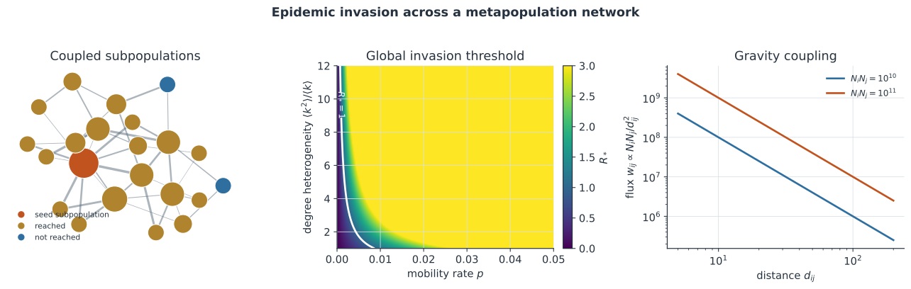
Reaction–diffusion metapopulations#
Model a set of subpopulations sitting on the nodes of a mobility network with degree distribution . Inside each node, individuals run a local reaction — an SIR or SIS epidemic — while individuals diffuse along the edges to neighboring nodes at some per-capita mobility rate (Colizza & Vespignani 2007, Nat. Phys.). The state is the number of susceptible, infectious, and recovered individuals in every node, and the dynamics couple local transmission to between-node transport. This is the theory behind global spread models: the reaction–diffusion picture of continuous space becomes a discrete network when space is a set of cities joined by flights.
Two thresholds, not one#
Local growth is governed by the familiar basic reproduction number: a subpopulation sustains an outbreak only if . Between-subpopulation spread is governed by a separate quantity, the global invasion threshold , defined as the expected number of subpopulations seeded by one already-infected subpopulation (Colizza & Vespignani 2007, Phys. Rev. Lett.). The metapopulation is invaded only when
A disease can clear the local bar and fail the global one: it burns through the seed city but sends too few infected travelers onward to ignite a second city. Raising is not enough; the pathogen also has to move.
What sets R*#
During a local outbreak of size proportional to , a node exports infected individuals to each neighbor at a rate set by the mobility and the number of residents. Summing the seedings a node delivers over the course of its outbreak gives a threshold of the schematic form
where is the mean subpopulation size and measures degree heterogeneity. Three levers raise : faster mobility , larger subpopulations (bigger outbreaks export more), and more heterogeneous mobility. In a scale-free network the second moment is large, so hubs make the metapopulation far easier to invade — heterogeneity lowers the mobility needed to cross .
Gravity and radiation coupling#
The mobility rates are not uniform. Empirically, the flux of travelers between two places follows a gravity model,
with flux growing in the product of the two population sizes and decaying with distance . Large, close cities exchange the most travelers and seed each other first, which is why epidemics tend to reach big hubs early regardless of geographic proximity. The radiation model is a parameter-free alternative that predicts commuting flux from the population lying within the radius between origin and destination.
A worked example#
Take a scale-free mobility network with local , so every subpopulation would sustain an outbreak on its own. At a mobility rate of per individual per step, the outbreak stays trapped in the seed subpopulation: the expected number of onward seedings is below one, so . Raise mobility to and each infected subpopulation now exports enough travelers to seed several neighbors before its own outbreak fades, so and the epidemic sweeps the whole network. The local reproduction number never changed; only the mobility crossed the global invasion threshold.
In code#
We build a small metapopulation on a scale-free graph, run a discrete SIR reaction with between-node mobility seeded in one subpopulation, and count how many subpopulations experience a real outbreak below and above the invasion threshold.
R#
library(igraph)

set.seed(1834)
G <- sample_pa(40, m = 2, directed = FALSE)
nb <- adjacent_vertices(G, V(G))
n <- 40; M <- 3000; beta <- 0.9; gamma <- 0.3

run <- function(p, steps = 120) {
  S <- rep(M, n); I <- rep(0, n); R <- rep(0, n)
  S[1] <- M - 20; I[1] <- 20
  for (t in seq_len(steps)) {
    ni <- rbinom(n, S, 1 - exp(-beta * I / M))
    nr <- rbinom(n, I, gamma)
    S <- S - ni; I <- I + ni - nr; R <- R + nr
    for (comp in c("S", "I", "R")) {
      x <- get(comp); leave <- rbinom(n, x, p); x <- x - leave
      for (i in seq_len(n)) if (leave[i] > 0) {
        k <- nb[[i]]
        x[k] <- x[k] + rmultinom(1, leave[i], rep(1 / length(k), length(k)))
      }
      assign(comp, x)
    }
  }
  sum(R > 0.02 * M)
}
sapply(c(5e-5, 1e-3), run)   # reached below vs above invasion
Python#
import numpy as np
import networkx as nx
import polars as pl

G = nx.barabasi_albert_graph(40, 2, seed=1834)   # scale-free mobility net
nbrs = [list(G[i]) for i in G.nodes()]
n, M = G.number_of_nodes(), 3000                 # subpops, individuals each
beta, gamma = 0.9, 0.3                            # local R0 = beta/gamma = 3


def run(p, steps=120):
    rng = np.random.default_rng(1834)
    S = np.full(n, M); I = np.zeros(n, int); R = np.zeros(n, int)
    S[0], I[0] = M - 20, 20                       # seed one subpopulation
    for _ in range(steps):
        newinf = rng.binomial(S, 1 - np.exp(-beta * I / M))
        newrec = rng.binomial(I, gamma)
        S -= newinf; I += newinf - newrec; R += newrec
        for comp in (S, I, R):                    # mobility: leave, then split
            leave = rng.binomial(comp, p)
            comp -= leave
            for i in range(n):
                if leave[i] and nbrs[i]:
                    share = rng.multinomial(leave[i], [1 / len(nbrs[i])] * len(nbrs[i]))
                    for j, c in zip(nbrs[i], share):
                        comp[j] += c
    return int((R > 0.02 * M).sum())              # subpops with a real outbreak


rows = [{"mobility_p": p, "subpops_reached": run(p)} for p in (5e-5, 1e-3)]
print(pl.DataFrame(rows))
shape: (2, 2)
┌────────────┬─────────────────┐
│ mobility_p ┆ subpops_reached │
│ ---        ┆ ---             │
│ f64        ┆ i64             │
╞════════════╪═════════════════╡
│ 0.00005    ┆ 1               │
│ 0.001      ┆ 39              │
└────────────┴─────────────────┘
Julia#
using Graphs, Distributions, Random

function run(p; steps = 120)
    rng = MersenneTwister(1834)
    G = barabasi_albert(40, 2; rng = rng)
    n, M, beta, gamma = 40, 3000, 0.9, 0.3
    S = fill(M, n); I = zeros(Int, n); R = zeros(Int, n)
    S[1] = M - 20; I[1] = 20
    for _ in 1:steps
        ni = [rand(rng, Binomial(S[i], 1 - exp(-beta * I[i] / M))) for i in 1:n]
        nr = [rand(rng, Binomial(I[i], gamma)) for i in 1:n]
        S .-= ni; I .+= ni .- nr; R .+= nr
        for comp in (S, I, R)
            for i in 1:n
                leave = rand(rng, Binomial(comp[i], p))
                comp[i] -= leave
                k = neighbors(G, i)
                isempty(k) && continue
                share = rand(rng, Multinomial(leave, fill(1 / length(k), length(k))))
                comp[k] .+= share
            end
        end
    end
    count(R .> 0.02 * M)
end

[run(p) for p in (5e-5, 1e-3)]   # reached below vs above invasion
Why it matters#
The invasion threshold explains why local control is not the whole story: a pathogen with everywhere can still be stopped from going global if travel is slow or evenly spread, and can be tipped over by air travel that concentrates flux through a few hubs. It reframes containment around mobility — travel restrictions, border screening, cordons — as acting on a different threshold than vaccination, which acts on local . The heterogeneity term is why real epidemics seed large, well-connected cities first and why scale-free mobility makes global spread so hard to prevent.