Source-Sink Dynamics

Not every patch that holds animals is pulling its weight. A source produces more offspring than it loses and exports the surplus; a sink loses more than it produces and persists only because immigrants keep arriving. Pulliam’s insight is that a sink can hold most of the population and still never sustain itself, so abundance is a poor guide to importance and eliminating the source, not the sink, is what ends persistence.

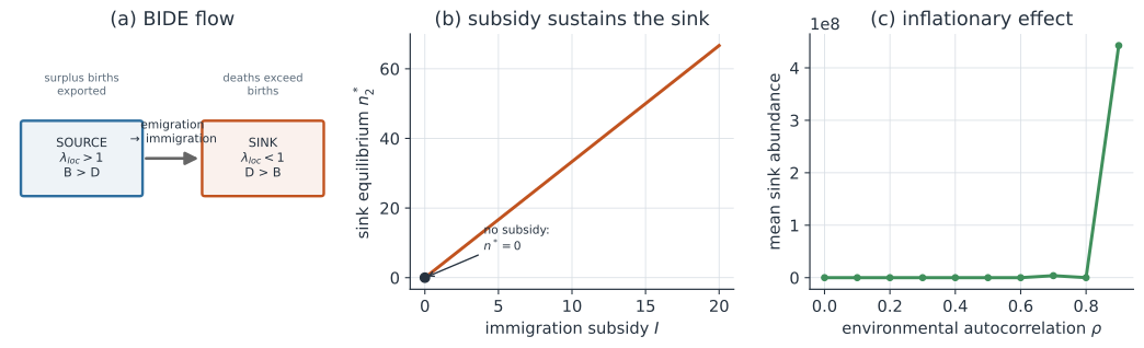
Three panels: a two-patch source-to-sink flow diagram annotated with the BIDE terms; sink equilibrium abundance rising linearly with the immigration subsidy from a starting value of zero; and the inflation of a would-be-sink metapopulation as environmental autocorrelation increases.

BIDE and the per-patch growth rate

Track a local population through four flows: Births, Immigration, Deaths, and Emigration. Stripping away the movement terms leaves the local demography, and the local finite rate of increase $\lambda_{\text{loc}}$ compares births to deaths in isolation, with no immigration. A patch is a source if it could grow on its own,

$\lambda_{\text{loc}} > 1 \quad (\text{births exceed deaths}),$

and a sink if it could not,

$\lambda_{\text{loc}} < 1 \quad (\text{deaths exceed births}).$

Pulliam (1988, American Naturalist 132:652-661, doi:10.1086/284880) built the framework on exactly this BIDE bookkeeping, and it is the demographic accounting that metapopulation models assume when they let patches differ in quality.

A sink persists only on subsidy

Consider a sink receiving a steady immigration subsidy $I$ each generation while its own numbers decay at the local rate $\lambda_2 < 1$ ,

$n_2(t+1) = \lambda_2\, n_2(t) + I.$

Its equilibrium abundance is

$n_2^* = \frac{I}{1 - \lambda_2}.$

Two things follow. With no immigration, $I = 0$ , the equilibrium is $n_2^* = 0$ : the sink cannot maintain itself and blinks out. With immigration, $n_2^*$ can be large, sitting far above its no-subsidy equilibrium of zero and rising in proportion to the subsidy, so a crowded patch may be nothing but a well-fed sink. This is why abundance misleads: counting bodies tells you where individuals accumulate, not where they are produced.

Reproductive-value weighting

If abundance is the wrong currency, the right one is reproductive value. Each patch’s contribution to the whole-metapopulation growth rate should be weighted by the reproductive value of the individuals it holds, not by their headcount. Individuals crowded into a sink have low reproductive value because most of their potential descendants die there without breeding, so a sink can hold half the population yet contribute almost nothing to future generations. The metapopulation grows or declines according to the reproductive-value-weighted sum across patches, which is dominated by the sources.

Environmental fluctuation and inflation

The source-sink split assumes fixed rates, but real environments fluctuate, and fluctuation plus dispersal can rescue patches that are sinks on average. Gonzalez & Holt (2002, PNAS 99:14872-14877, doi:10.1073/pnas.232589299) showed that when a patch’s growth rate varies over time with positive autocorrelation, immigrants arriving during good runs get amplified before the next bad run, so the long-run mean abundance is inflated above what the average rate alone predicts. This inflationary effect connects source-sink logic to asynchrony and the inflationary effect: temporal variation, not just spatial structure, can let a set of average-sink patches persist as a metapopulation.

Disease relevance

The framework maps directly onto multi-host disease systems. A reservoir host or habitat where the pathogen maintains $\lambda_{\text{loc}} > 1$ (its local $R_0$ exceeds one) is a source, while a spillover host where the pathogen cannot sustain transmission on its own ( $R_0 < 1$ ) is a sink that only carries infection because of repeated introduction from the reservoir. The control implication is the same as the ecological one: culling or vaccinating the spillover sink treats symptoms, while targeting the reservoir source is what removes the subsidy that sustains the whole system.

A worked example

Couple a self-regulating source to a decaying sink. The source grows logistically toward carrying capacity $K = 100$ with intrinsic rate $r = 0.8$ and exports a fraction $m = 0.2$ of its numbers each step; the sink decays at $\lambda_2 = 0.7$ and receives that emigration as immigration. At equilibrium the source settles at $n_1^* = K(1 - m/r) = 75$ , exports a flow of $m\,n_1^* = 15$ , and the sink holds $n_2^* = 15/(1 - 0.7) = 50$ even though its own births fall short of its deaths. Cut the link and the sink collapses to zero, while the source is untouched: the sink holds two-fifths of the whole population but produces none of it.

In code

We iterate the two-patch difference model to equilibrium and report each patch’s abundance and the net flow, showing the sink survives only on subsidy.

R

K <- 100; r <- 0.8; m <- 0.2; lam2 <- 0.7
n1 <- 1; n2 <- 0
for (t in 1:2000) {
  e  <- m * n1                       # emigration from the source
  n1 <- n1 + r * n1 * (1 - n1 / K) - e
  n2 <- lam2 * n2 + e                # sink: local decline plus immigration
}
c(source = n1, sink = n2, flow = m * n1, sink_no_subsidy = 0)

Python

import numpy as np

K, r, m, lam2 = 100.0, 0.8, 0.2, 0.7   # source K, growth, dispersal, sink rate
n1, n2 = 1.0, 0.0
for _ in range(2000):
    e = m * n1                          # emigration from source
    n1 = n1 + r * n1 * (1 - n1 / K) - e
    n2 = lam2 * n2 + e                  # sink: local decline plus immigration
flow = m * n1
print("source abundance n1* =", round(n1, 2))
print("sink abundance   n2* =", round(n2, 2))
print("net flow source -> sink =", round(flow, 2))
print("sink without subsidy    =", round(0.0, 2))

source abundance n1* = 75.0
sink abundance   n2* = 50.0
net flow source -> sink = 15.0
sink without subsidy    = 0.0

Julia

K, r, m, lam2 = 100.0, 0.8, 0.2, 0.7
n1, n2 = 1.0, 0.0
for t in 1:2000
    e  = m * n1                         # emigration from the source
    n1 = n1 + r * n1 * (1 - n1 / K) - e
    n2 = lam2 * n2 + e                  # sink: local decline plus immigration
end
(source = n1, sink = n2, flow = m * n1, sink_no_subsidy = 0.0)

Why it matters

Source-sink dynamics reframes where to look and where to act: the patch with the most individuals may contribute the least to persistence, and protecting or attacking it can miss the point entirely. For conservation it warns that a crowded sink is not a healthy population, and that reproductive value, not census size, is the currency of importance. For disease control it says the same thing in reverse: chasing infections in spillover hosts leaves the reservoir source untouched, so persistence continues, and the metapopulation view combined with reproductive value is what turns a map of where cases appear into a plan for where to intervene.