Species Distribution Models: Presence-Only Data

Where can a mosquito vector, a reservoir host, or a pathogen actually live? A species distribution model (SDM, or ecological niche model) answers that by learning how occurrence depends on the environment — temperature, rainfall, land cover — and projecting it across a map. The hardest and most common data regime is presence-only: museum specimens, GBIF records, trap catches, case reports — a pile of places the species was found, with no record of where anyone looked and found nothing. This page handles that case; its companion handles surveyed presence–absence data.

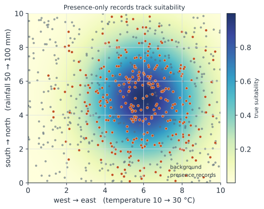
Figure 1. A landscape whose environmental suitability (shaded, from a unimodal temperature-and-rainfall niche) peaks in a central band. Presence records concentrate where suitability is high; a background sample is spread across the whole landscape. The model learns the niche by contrasting the two.

The presence-only problem#

You cannot fit “presence versus absence” when you have no absences. A record that a species was collected at a site tells you the environment there is adequate; the silence everywhere else is ambiguous — nobody looked, or they looked and missed, or it is genuinely unsuitable. Worse, occurrence records carry sampling bias: they cluster near roads, cities, and field stations, so raw records describe where people go as much as where the species is.

Background points and the point-process view#

The workhorse fix is to contrast the presences against background (or “pseudo-absence”) points — a sample of the environment available across the whole landscape. This does not pretend the background points are absences; it asks a subtly different question: where the species occurs, how does the environment differ from what is available on average?

Formally, presence-only data are a realization of an inhomogeneous Poisson point process with intensity

$\lambda(z) = \exp\!\big(\alpha + \beta^\top z\big),$

where $z$ is the environment at a location. Fitting Maxent — the most widely used presence-only method — is mathematically equivalent to fitting this Poisson process, and to a weighted logistic regression of presences (1) against background (0) with the background heavily up-weighted (Renner & Warton 2013; Fithian & Hastie 2013). So the same logistic-regression machinery used elsewhere on this site, pointed at presence-versus-background, is a niche model.

What you can — and cannot — estimate#

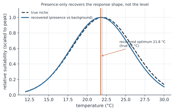
The point process makes the limits precise. The shape of the response (the $\beta$ ’s — the optimum temperature, the rainfall tolerance) is identifiable and is what an SDM is really after. The intercept $\alpha$ — the absolute occurrence rate, i.e. prevalence or abundance — is not identifiable from presence-only data alone: doubling the true density and halving the sampling effort produce identical records.

Warning

Presence-only models estimate relative suitability, not probability of occurrence. Reporting a Maxent “probability” as if it were $P(\text{present})$ is a standard error — the absolute level depends on unknown sampling effort. To pin down prevalence you need presence–absence or presence-and-effort data. And because records are spatially biased, sample the background with the same bias (a “target-group” background) or include a bias covariate, or the model learns the sampling pattern instead of the niche.

A worked example: recovering a thermal niche#

We simulate a species whose true suitability is unimodal in temperature (optimum $22^\circ$ C) and rainfall (optimum $75$ mm), draw presence records by thinning a Poisson process by suitability, add a background sample, and fit the equivalent presence-versus-background logistic model. It recovers the niche optimum closely — from occurrence records and background alone (Figure 2).

Figure 2. The fitted temperature response (relative suitability, rainfall held at its optimum) against the true niche. The presence-versus-background model recovers the unimodal shape and the optimum near 22°C, though the absolute height is not identified.

Python

import numpy as np
from sklearn.linear_model import LogisticRegression

rng = np.random.default_rng(1)
temp = lambda x: 10 + 2.0 * x                    # environment over the landscape
rain = lambda y: 50 + 5.0 * y
t_opt, t_w, r_opt, r_w = 22.0, 4.0, 75.0, 12.0
suit = lambda x, y: np.exp(-((temp(x) - t_opt) ** 2) / (2 * t_w**2)
                           - ((rain(y) - r_opt) ** 2) / (2 * r_w**2))

# presence records: thin a uniform Poisson process by suitability
cand = rng.uniform(0, 10, size=(20000, 2))
pres = cand[rng.uniform(size=len(cand)) < suit(cand[:, 0], cand[:, 1])][:300]
bg = rng.uniform(0, 10, size=(3000, 2))          # background sample of the landscape

def feats(P):
    t, r = temp(P[:, 0]), rain(P[:, 1])
    return np.column_stack([t, t**2, r, r**2])

X = np.vstack([feats(pres), feats(bg)])
y = np.r_[np.ones(len(pres)), np.zeros(len(bg))]
w = np.r_[np.ones(len(pres)), np.full(len(bg), len(pres) / len(bg))]  # IPP weights
Xs = (X - X.mean(0)) / X.std(0)
m = LogisticRegression(C=1e6, max_iter=5000).fit(Xs, y, sample_weight=w)

b = m.coef_[0] / X.std(0)                         # de-standardize the coefficients
print(f"recovered temp optimum {-b[0] / (2 * b[1]):.1f}  (true {t_opt})")
print(f"recovered rain optimum {-b[2] / (2 * b[3]):.1f}  (true {r_opt})")
print(f"{len(pres)} presence records vs {len(bg)} background points; "
      f"intercept (prevalence) is NOT identifiable")

recovered temp optimum 21.8  (true 22.0)
recovered rain optimum 73.7  (true 75.0)
300 presence records vs 3000 background points; intercept (prevalence) is NOT identifiable

In code#

R#

library(maxnet)           # Maxent as a regularized presence-vs-background GLM
# p: 1 for presences, 0 for background; env: data frame of covariates
fit <- maxnet(p, env, f = maxnet.formula(p, env, classes = "lq"))  # linear+quadratic
plot(fit, "temp", type = "cloglog")   # the fitted temperature response
# glmnet / the 'ppmlasso' package fit the identical point-process model directly

Julia#

Julia

using GLM, DataFrames
# presence-vs-background logistic regression = the Poisson point-process model;
# weight background rows by n_presence / n_background to match the IPP likelihood
fit = glm(@formula(y ~ temp + temp^2 + rain + rain^2), df, Binomial(), wts = w)

Why it matters#

Presence-only niche models underpin much of the mapping of vector-borne and zoonotic disease risk: the projected range of Aedes and Anopheles mosquitoes under climate change, the reservoirs of Ebola or Lassa, the suitability surface for a newly emerging pathogen — almost always built from opportunistic occurrence records because systematic surveys do not exist. Understanding that these models estimate relative suitability, are equivalent to a Poisson point process, and are corrupted by sampling bias unless you correct for it, is the difference between a defensible risk map and a map of where naturalists happen to travel.