Remote Sensing, Object Counting, and Outbreak Detection
Sometimes the most useful epidemiological signal is not a case report but a proxy for one — a sign that people are behaving as if sick before any of them are counted. Hospital activity is one such proxy, and it is visible from above: a full parking deck is a crude, real-time gauge of how many people are seeking care. This page ties three threads together — remote sensing (imagery of the physical world), machine-learning object counting (turning that imagery into numbers), and outbreak detection (turning numbers into an alarm) — using a hospital parking deck as the worked example. It is deliberately a cautionary tale as much as a method: the pipeline is easy to build and easy to fool.
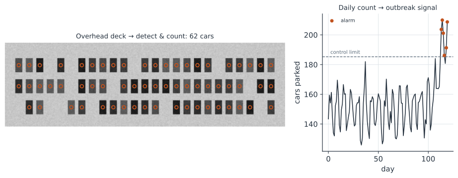
From classification to counting#
The convolutional networks page asked what is in this image?. Counting asks a harder question — how many, and where? — which is the task of object detection: locate every instance of a class and draw a box around it. Modern detectors (the YOLO family, Faster R-CNN, RetinaNet) are CNNs with two heads on top of a shared backbone, one predicting a box’s location and one its class, trained on images with boxes drawn by hand. Count the boxes of class “car” and you have counted the cars. For clean, synthetic imagery you can cheat with classical computer vision — threshold the image, label the connected components, keep the car-sized ones — but that shortcut works only because we built the image and already know a car is a dark blob. On real, messy overhead photos the rule is not obvious, so the meaningful approach is to train a model on labelled examples of what a car looks like and then apply it, which is what the next section and the runnable code do.
Training a detector: label, learn, apply#
Every supervised detector, from this page’s toy CNN to YOLO, follows the same three steps.
Label. Assemble examples of the target and of everything else — image patches (or hand-drawn boxes) marked “car” and “not car”. This is the expensive, human part, and the quality and representativeness of the labels cap everything downstream: a detector only ever learns the cars it was shown.
Learn. Train a model — here a small convolutional network — to map a patch to the probability that it contains a car, by minimizing classification loss on the labelled set. Hold out a validation split the model never trains on and judge it there; high training accuracy with poor validation accuracy means it memorized the examples instead of learning the concept. Because the network learns its own features — dark rectangular shape, size, contrast — it generalizes to cars it has never seen, which a fixed threshold cannot.
Apply. Slide the trained classifier across a new, unlabelled image, score every location, then collapse each cluster of overlapping high-scoring windows into a single detection (non-maximum suppression) and count them. This “train once, apply anywhere” is exactly what makes the model reusable across days, decks, and cameras — and it is the workflow the code below implements end to end.
Remote sensing as a data source#
Remote sensing is measurement at a distance — satellites, aircraft, drones, and fixed cameras imaging the physical world. Epidemiology has long borrowed from it: satellite-derived rainfall, temperature, and vegetation feed vector-borne disease and climate-forcing models, and night-time lights serve as a proxy for economic activity and population. What is newer is using high-resolution overhead imagery of human activity — how full a parking lot is, how busy a road is — as a near-real-time behavioural signal. The appeal is that it is passive, needs no cooperation from the people it observes, and can update daily; the peril, as below, is that it measures behaviour, and behaviour has many causes.
Getting the imagery#
A practical snag is licensing: Google Maps/Earth, Bing, and Esri imagery can be viewed but not redistributed, so they cannot supply an image you publish or bake into a reproducible pipeline. License-clean sources do exist, and for counting cars you need roughly 15–60 cm resolution.
- Government aerial orthophotos are the best route for a specific facility: US state and county GIS open-data portals (for example NC OneMap) publish 3–6 inch orthoimagery that is usually public domain, and USGS EarthExplorer serves nationwide NAIP imagery (~0.6 m, public domain).
- Openly-licensed imagery: OpenAerialMap hosts CC-licensed aerial and drone imagery, and the Maxar Open Data program releases high-resolution scenes for disaster events.
- Your own drone (where permitted) gives imagery you fully own, at a resolution you choose.
- Coarse free satellites won’t work: Sentinel-2 (10 m) and Landsat (15–30 m) cannot resolve individual cars — use them for climate and land cover, not counting.
- Labelled training data: to train a detector, overhead-vehicle datasets such as CARPK (drone images of parking lots with per-car annotations), COWC, and xView provide ready-made examples.
The proxy chain, and its assumptions#
The logic linking a parking count to disease is a chain of assumptions, each of which can break: Reading a rise in cars as a rise in disease assumes that occupancy tracks visits (not staff shifts, construction, or a nearby event), that visits track care-seeking (not elective procedures or visitors), that care-seeking tracks illness (not fear or a policy change), and that the illness is the one you care about. None of these holds exactly, and several fail badly under exactly the conditions — a novel outbreak, a public scare — when you most want the signal. The count is therefore best treated as one weak, non-specific indicator to be corroborated against specific data (syndromic surveillance, test positivity), never as a standalone diagnosis of an outbreak.
From counts to an alarm#
Once each day yields a count, you have a time series, and detecting an outbreak becomes detecting an aberration in that series — the subject of aberration detection. The simplest detector is a control chart: estimate a baseline mean and standard deviation from a quiet period, and flag any day that exceeds an upper control limit such as , as on the right of the figure. More robust versions account for the day-of-week and seasonal structure (a deck is fuller on weekdays), use the EWMA or CUSUM to catch gradual rises, or feed the multivariate signal to a variational autoencoder whose reconstruction error flags the unusual day. The same proper scoring and validation discipline as any forecast applies: an alarm is a prediction, and it must be checked against what actually happened.
A practical example: the Eden Terrace deck#
Make it concrete with a real facility — the Eden Terrace parking deck serving a hospital campus, a long two-to-three-row deck plainly visible in overhead maps. A synthetic deck built to that layout, shown at three occupancy levels and run through the same crude dark-blob detector, illustrates the idea end to end: the count falls from a packed deck to a nearly empty one, exactly the occupancy signal a surveillance pipeline would track over time.
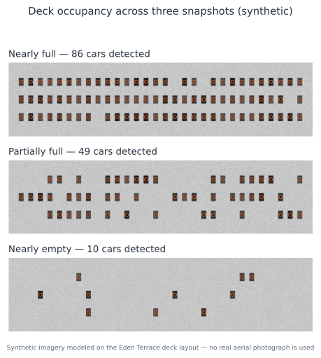
As Figure 2 shows, even a threshold-and-count heuristic separates a full deck from an empty one cleanly. Now imagine acquiring such an image daily, and suppose the deck holds about cars and typically sits near occupied on a weekday; if over two weeks the daily count climbed past — above a control limit built from the prior quiet months — that would be an alarm worth a look. It might reflect a wave of respiratory visits, or it might be a staff-parking change, a nearby road closure pushing cars onto the deck, a home football weekend, or simply better weather. The figure and the runnable code below both use a synthetic deck of the Eden Terrace layout — the pipeline is real and reproducible, the imagery is modeled rather than a real (license-restricted) aerial photograph, and every caveat in the next section applies with full force.
This example is illustrative only. The detector is a crude threshold-and-count heuristic (a real system would use the trained detector below), the deck and its occupancy are synthetic rather than a validated daily time series, and nothing has been checked against actual case data. Nothing here should be read as a claim that parking counts detected, or could detect, any specific outbreak.
What the literature actually shows#
The best-known attempt at exactly this was a 2020 analysis arguing that satellite images of Wuhan hospital parking lots, together with Baidu searches for symptoms, hinted at elevated activity in the autumn of 2019 (Nsoesie et al.). It drew wide attention and equally wide criticism: the parking lots were confounded by seasonality, construction, and image-quality differences, the comparison images were sparse, and the search-term signal was weak — a textbook case of an intriguing proxy that cannot bear the causal weight placed on it. The honest lesson is not that overhead imagery is useless but that it is suggestive, not confirmatory: it can flag where to look, and it fails when used as evidence on its own. Remote sensing has firmer footing elsewhere in the field — night-time lights and mobility for population and movement, satellite climate variables for vector suitability — where the proxy chain is shorter and better validated.
In code#
Python#
Step 1–2: label patches and train a detector. We build the overhead deck we ultimately want to count, then assemble a labelled set of “car” and “not-car” patches and train a small CNN to tell them apart, judging it on a held-out validation split.
import numpy as np, torch, torch.nn as nn
rng = np.random.default_rng(7)
torch.manual_seed(0)

H, W = 96, 320                                       # the deck we want to count
deck = np.full((H, W), 0.78)                         # light asphalt
planted = 0
for ry in (26, 50, 74):                              # three rows of bays
    for cx in range(16, W - 12, 12):
        if rng.random() < 0.82:                      # ~82% of bays occupied
            planted += 1
            deck[ry - 5:ry + 5, cx - 3:cx + 3] = rng.choice([.12, .18, .24, .30])
deck = np.clip(deck + 0.02 * rng.standard_normal((H, W)), 0, 1)

def patch(is_car):                                   # a 16x10 labelled example
    p = np.full((16, 10), 0.78)
    if is_car:                                        # a jittered dark car blob
        dy, dx = rng.integers(-2, 3), rng.integers(-1, 2)
        p[3 + dy:13 + dy, 2 + dx:8 + dx] = rng.choice([.12, .18, .24, .30])
    return np.clip(p + 0.03 * rng.standard_normal((16, 10)), 0, 1)

Xp = np.stack([patch(i % 2 == 0) for i in range(1000)])          # alternate car/bg
yp = np.array([[1.0 - i % 2] for i in range(1000)], dtype=np.float32)   # 1 = car
Xt = torch.tensor(Xp[:, None], dtype=torch.float32)
yt = torch.tensor(yp)
tr, va = slice(0, 800), slice(800, 1000)             # train / validation split

net = nn.Sequential(                                 # a tiny "is this a car?" CNN
    nn.Conv2d(1, 8, 3, padding=1), nn.ReLU(), nn.MaxPool2d(2),
    nn.Conv2d(8, 16, 3, padding=1), nn.ReLU(), nn.AdaptiveMaxPool2d(1),
    nn.Flatten(), nn.Linear(16, 1))
opt = torch.optim.Adam(net.parameters(), lr=0.01)
for epoch in range(120):
    opt.zero_grad()
    loss = nn.functional.binary_cross_entropy_with_logits(net(Xt[tr]), yt[tr])
    loss.backward(); opt.step()
acc = lambda s: ((net(Xt[s]) > 0).float() == yt[s]).float().mean().item()
print(f"trained on 800 patches | train acc {acc(tr):.2f}  val acc {acc(va):.2f}")
trained on 800 patches | train acc 1.00 val acc 1.00
Step 3: apply the trained detector to the deck and count. Slide it over the image, keep windows it scores as cars, and suppress overlapping detections so each car is counted once.
from scipy.ndimage import maximum_filter
ys, xs = list(range(0, H - 16 + 1, 4)), list(range(0, W - 10 + 1, 4))
wins = np.stack([deck[y:y + 16, x:x + 10] for y in ys for x in xs])
with torch.no_grad():
    score = torch.sigmoid(net(torch.tensor(wins[:, None],
                                           dtype=torch.float32))).numpy()
S = score.reshape(len(ys), len(xs))                  # a score map over the deck

# non-max suppression = keep local maxima; the footprint spans one car
# (tall enough to merge a car's own overlapping windows, narrow enough to
#  keep neighbouring cars in a row distinct)
peaks = (S == maximum_filter(S, size=(3, 3))) & (S > 0.9)
print(f"detector counted {int(peaks.sum())} cars (planted {planted})")
detector counted 62 cars (planted 62)
Turning the daily count into an alarm is a control chart: baseline from a quiet period, then flag days above .
days = np.arange(120)
base = 150 + 14 * np.sin(2 * np.pi * days / 7)      # weekly rhythm around 150
counts = base + rng.normal(0, 6, 120)
counts[104:] += np.linspace(0, 62, 16)              # a two-week surge
mu, sd = counts[:100].mean(), counts[:100].std()    # baseline from quiet weeks
ucl = mu + 3 * sd                                    # upper control limit
alarm_days = days[counts > ucl]
print(f"baseline mean {mu:.0f}, control limit {ucl:.0f}")
print(f"alarm on days: {alarm_days.tolist()}")
baseline mean 150, control limit 184
alarm on days: [113, 114, 115, 116, 118, 119]
On real imagery you rarely train from scratch — you fine-tune a pretrained detector like YOLO (transfer learning) on a few hundred labelled overhead images, then apply it exactly as above (illustrative — it fetches model weights over the network, so it is shown, not run):
# no-run
from ultralytics import YOLO                        # a pretrained object detector

model = YOLO("yolov8n.pt")                           # COCO-pretrained weights
result = model("deck_2026-07-11.jpg", classes=[2])   # class 2 = "car"
print(f"{len(result[0].boxes)} cars detected")
R#
# Train a patch classifier with torch, then slide it over the image to count.
library(torch)
net <- nn_sequential(
  nn_conv2d(1, 8, 3, padding = 1), nn_relu(), nn_max_pool2d(2),
  nn_conv2d(8, 16, 3, padding = 1), nn_relu(), nn_adaptive_max_pool2d(1),
  nn_flatten(), nn_linear(16, 1))
# ... train net on labelled car/not-car patches, then apply over sliding windows
# (EBImage::bwlabel on a threshold is the no-training shortcut for clean images).
Julia#
# Flux to train the patch classifier; slide it over the image to count.
using Flux
net = Chain(Conv((3, 3), 1 => 8, relu, pad = 1), MaxPool((2, 2)),
            Conv((3, 3), 8 => 16, relu, pad = 1), GlobalMaxPool(),
            Flux.flatten, Dense(16 => 1, σ))
# ... train net on labelled car/not-car patches, then apply over sliding windows.
Confounders, privacy, and validation#
This idea lives or dies on three non-technical issues, and they deserve as much care as the model.
Confounding. A parking count responds to weather, holidays, day of week, staff schedules, construction, nearby events, and parking-policy changes far more reliably than to any single disease. Without adjusting for these — and without a specific comparison series — a rise is uninterpretable, and the risk of crying wolf (or missing a real signal buried in the noise) is high.
Privacy and ethics. Persistent overhead surveillance of a specific facility, even counting only cars, raises real concerns: it can expose sensitive patterns (who visits a clinic, when), and imagery good enough to see cars can often see people or plates. Aggregate to counts, avoid tracking individuals, respect the terms and copyright of the imagery source, and ask whether the public-health value justifies the surveillance at all.
Validation. A proxy is worthless until it is shown to track the thing you care about. That means correlating the count against real case or syndromic data over a long period, quantifying its lead time and false-alarm rate with proper scoring rules, and testing it prospectively before anyone acts on it. An unvalidated proxy that feels predictive is exactly how a confounded coincidence becomes a confident mistake.
Why it matters#
Activity proxies from remote sensing are a genuine addition to the surveillance toolkit — cheap, passive, and fast — and object-counting models make them usable at scale. At their best they are an early, non-specific tripwire that tells an epidemiologist where to point the specific instruments: test more here, pull the line list there. But every strength is shadowed by the proxy chain’s fragility, so the right posture is humility: treat the count as one weak signal among many, corroborate before believing, adjust for the obvious confounders, guard privacy, and validate against ground truth. Used that way — as a hypothesis generator feeding the aberration-detection and forecasting machinery, not replacing it — remote sensing ties the physical world to the epidemiological one without overpromising.