Uncertainty, Calibration, and Conformal Prediction

A prediction without honest uncertainty is a liability, nowhere more than in health, where a confident wrong answer can cost a life. A model that says “90% risk” should be right about nine times in ten it says so, and a forecast of next week’s cases should come with an interval that actually contains the truth about as often as it claims. This page covers three linked ideas that make predictions trustworthy: the two kinds of uncertainty a model faces, calibration so that probabilities mean what they say, and conformal prediction, which wraps any model in prediction sets that carry a mathematical coverage guarantee.

Two kinds of uncertainty#

Not all uncertainty is the same, and the distinction changes what you can do about it. Aleatoric uncertainty is irreducible noise in the world — two patients with identical records can have different outcomes — and no amount of data removes it; the best a model can do is report it honestly. Epistemic uncertainty is the model’s own ignorance, from limited or unrepresentative data, and it shrinks as you collect more or move back toward where the training data lived. The practical consequence is that a model should be more uncertain about a patient unlike any it trained on (high epistemic uncertainty) than about a typical one — and a model that is confidently wrong on out-of-distribution inputs, as many neural networks are, is failing to represent its epistemic uncertainty. Bayesian inference, deep ensembles, and Monte-Carlo dropout are the usual tools for estimating it.

Calibration#

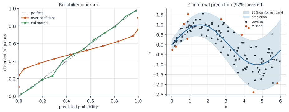
A probabilistic prediction is calibrated if it means what it says: among all the cases a model assigns probability $p$, a fraction close to $p$ should actually be positive. You check this with a reliability diagram (left of the figure): bin predictions by their stated probability and plot the observed frequency in each bin against the mean predicted probability; a calibrated model tracks the diagonal, while an over-confident one — predicting probabilities too close to 0 and 1 — bows away from it. The expected calibration error (ECE) summarizes the gap as a weighted average distance from the diagonal. Calibration is one half of a good forecast; the other is sharpness (confident, concentrated predictions), and a proper scoring rule like the Brier or log score rewards both at once. When a model discriminates well but is miscalibrated, you recalibrate it after the fact — Platt scaling (fit a logistic on its scores), isotonic regression (a nonparametric monotone fit), or temperature scaling for neural networks (divide the logits by a single learned scalar) — using a held-out set, which fixes the probabilities without touching the ranking. This is the same reasoning behind a diagnostic test’s predictive values: a score is only as useful as the real-world frequency it corresponds to.

Conformal prediction#

Calibration makes a probability honest; conformal prediction goes further and returns a set of outcomes guaranteed to contain the truth with a chosen probability — for any model, with no distributional assumptions, from finite data. The most common recipe is split (inductive) conformal. Set aside a calibration set the model did not train on, and for each of its points compute a nonconformity score — how surprising the true label is under the model, e.g. the absolute residual $|y - \hat f(x)|$ for regression. Take the $\lceil (n+1)(1-\alpha)\rceil / n$ empirical quantile $\hat q$ of those scores, and for a new input output the prediction set of all labels whose nonconformity is $\le \hat q$ — an interval $\hat f(x) \pm \hat q$ for regression, or a set of plausible classes for classification. Under only the assumption that the data are exchangeable, this set satisfies a finite-sample guarantee, $$\mathbb{P}\bigl(Y_{\text{new}} \in \hat C(X_{\text{new}})\bigr) \ge 1 - \alpha, \tag{1}$$ the marginal coverage shown holding on the right of the figure, where a 90%-target band covers about 90% of held-out points. Making the score adaptive — for instance dividing the residual by a local noise estimate — lets the interval widen where the data are noisy and tighten where they are clean, as the figure’s band does, without breaking the guarantee.

A worked example#

Fit any regression model, then hold out $500$ calibration points and record each absolute residual $|y_i - \hat f(x_i)|$. For 90% coverage ($\alpha = 0.1$), the conformal quantile is the $\lceil 501 \times 0.9\rceil = 451$st smallest of those $500$ residuals — say it is $0.62$. Then for any new $x$, the interval $\hat f(x) \pm 0.62$ is guaranteed to contain the true $y$ at least 90% of the time over future exchangeable data — regardless of whether the model is a linear fit, a random forest, or a neural network, and regardless of the noise distribution. The price is only a held-out calibration set and the honesty to report an interval instead of a point.

In code#

Python#

Split-conformal prediction turns any model’s residuals into an interval with guaranteed coverage — here the coverage lands near the 90% target on held-out data:

import numpy as np
rng = np.random.default_rng(0)

f = lambda x: np.sin(x)                          # the (already fitted) mean model
n = 1000
x = rng.uniform(0, 6, n)
y = f(x) + rng.normal(0, 0.3, n)                 # homoscedastic noise for simplicity
cal, test = slice(0, 500), slice(500, 1000)      # calibration / test split

alpha = 0.10
scores = np.abs(y[cal] - f(x[cal]))              # nonconformity = absolute residual
k = int(np.ceil((500 + 1) * (1 - alpha)))        # finite-sample quantile rank
q = np.sort(scores)[k - 1]
covered = np.abs(y[test] - f(x[test])) <= q      # is the truth inside f(x) ± q ?
print(f"interval half-width q = {q:.3f}")
print(f"target coverage {100*(1-alpha):.0f}%, achieved {100*covered.mean():.1f}%")

interval half-width q = 0.503
target coverage 90%, achieved 90.0%

Calibration is checked with a reliability curve and fixed by recalibration:

from sklearn.calibration import calibration_curve
p_true = rng.uniform(0, 1, 3000)
labels = (rng.uniform(size=3000) < p_true).astype(int)
logit = np.log(p_true / (1 - p_true))
p_over = 1 / (1 + np.exp(-1.8 * logit))          # sharpened logits = over-confident
frac, mean_pred = calibration_curve(labels, p_over, n_bins=10)
print(f"expected calibration error (over-confident): {np.mean(np.abs(frac - mean_pred)):.3f}")

expected calibration error (over-confident): 0.072

The mapie library wraps any scikit-learn model in conformal intervals, making the three-way train / conformalize / test split explicit — here around a random forest, again landing near the 90% target:

from sklearn.ensemble import RandomForestRegressor
from sklearn.model_selection import train_test_split
from mapie.regression import SplitConformalRegressor

X2 = rng.uniform(0, 6, (3000, 1))
y2 = f(X2.ravel()) + rng.normal(0, 0.3, 3000)
X_tr, X_rest, y_tr, y_rest = train_test_split(X2, y2, test_size=0.5, random_state=0)
X_conf, X_te, y_conf, y_te = train_test_split(X_rest, y_rest, test_size=0.5,
                                              random_state=0)

scr = SplitConformalRegressor(RandomForestRegressor(n_estimators=200, random_state=0),
                              confidence_level=0.9, prefit=False)
scr.fit(X_tr, y_tr)                            # 1. train the underlying model
scr.conformalize(X_conf, y_conf)               # 2. calibrate on a held-out split
_, y_int = scr.predict_interval(X_te)          # 3. 90% prediction intervals
lo, hi = y_int[:, 0, 0], y_int[:, 1, 0]
covered = (y_te >= lo) & (y_te <= hi)
print(f"target coverage 90%, achieved {100 * covered.mean():.1f}%")
print(f"mean interval width {np.mean(hi - lo):.2f}")

target coverage 90%, achieved 89.2%
mean interval width 1.17

R#

# probably for calibration; the conformalInference / probably packages for conformal.
library(probably)
cal_plot_breaks(data, truth = outcome, estimate = .pred_pos)   # reliability diagram
# split-conformal by hand: quantile of calibration-set residuals
q <- quantile(abs(y_cal - predict(model, x_cal)), 0.9, type = 1)

Julia#

# ConformalPrediction.jl wraps MLJ models with conformal guarantees.
using ConformalPrediction, MLJ
conf_model = conformal_model(model; coverage = 0.9)
mach = machine(conf_model, X, y) |> fit!
predict(mach, Xnew)     # returns prediction sets / intervals

Why it matters#

Uncertainty is the difference between a model that informs a decision and one that misleads it. A calibrated risk score can be compared against a treatment threshold and trusted to mean what it says; an outbreak forecast with valid intervals tells a public-health team how wide to plan for, not just a central guess; and conformal prediction gives even a black-box deep-learning model a coverage guarantee a decision-maker can rely on, without retraining it. The recurring caution is distribution shift: calibration and conformal coverage are promises about data that look like the calibration data, and a new variant, population, or season can void them — which is why honest uncertainty is paired with monitoring, and why every model on this site is asked to say not just what it predicts, but how much it should be believed.

Related#

• Proper Scoring Rules
• Diagnostic Testing and Screening
• Bayesian Inference
• Model Interpretability and SHAP
• Overfitting, Regularization, and Cross-Validation
• The Effective Reproduction Number and Forecasting
• Quantitative Methods