Critical Community Size and Epidemic Fade-Out

A deterministic model treats the number of infectious people as a smooth quantity that can dip to a fraction of one and bounce back, but real infections are whole individuals: once the last case recovers, transmission stops until someone reintroduces the pathogen. After a big epidemic, susceptibles are used up and cases crash to a deep trough, and in a small population that trough can hit exactly zero and break the chain of transmission. The critical community size (CCS) is the population above which births refill the susceptible pool fast enough for the infection to survive its troughs, and below which it repeatedly fades out.

$Three panels: fraction of time with zero cases rising sharply as population size falls below the measles critical community size; one small-population run fading out in the post-epidemic trough while a large-population run persists; and the probability that a single major epidemic burns out declining as the reproduction number grows.$

The trough problem

Run the SIR model with vital dynamics deterministically and it settles toward an endemic equilibrium through damped oscillations: epidemics overshoot, susceptibles are depleted, prevalence falls to a trough, births slowly replenish susceptibles, and the next epidemic builds. The deterministic trough is small but positive, so the model always recovers.

Demographic stochasticity changes the story. Infectious individuals are discrete, and in the trough there may be only a handful of them, each of whom recovers or dies on a random clock. If they all clear before a new case is generated, the number infectious reaches zero and stays there, because nothing in a closed population creates infection from nothing. Persistence is therefore a race: susceptible replenishment by births must lift transmission back above threshold before the stochastic trough empties. This is the machinery of demographic stochasticity and the Gillespie algorithm applied to its most famous consequence.

What sets the critical community size

The depth of the trough, and so the chance of extinction, depends on a few quantities.

Population size. Larger populations carry more infectious individuals through the trough, so the probability that all of them clear at once is smaller.
Birth rate. Faster susceptible replenishment shortens the interepidemic period and shallows the trough, lowering the CCS.
Infectious period. A longer infectious period keeps each case transmitting longer, which helps bridge the gap between epidemics.
Epidemic amplitude. A highly transmissible pathogen burns through susceptibles quickly and overshoots hard, producing a deeper trough that is easier to empty.

Bartlett estimated the measles CCS empirically at roughly 250,000–300,000 people by relating the frequency of fade-outs in towns and cities to their size (Bartlett 1957). Below that size measles could not persist and depended on reintroduction; above it, transmission was continuous. Keeling and Grenfell reproduced the threshold from a mechanistic model, showing that getting the CCS right requires realistic handling of the trough — the deterministic mean-field prediction is far too low, and the details of how infection is distributed among individuals matter (Keeling and Grenfell 1997).

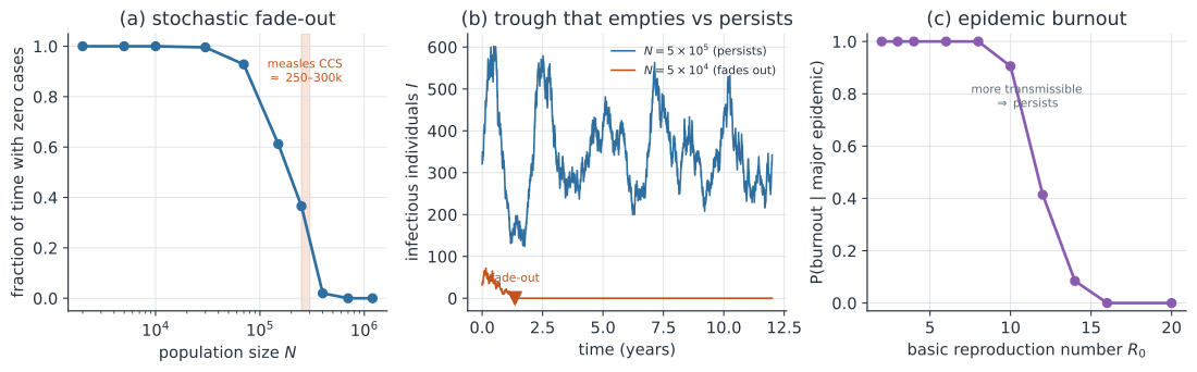
Panel (a) shows the signature: the fraction of time a population spends with zero cases stays near zero for large populations and rises sharply as the population falls through the CCS band. Panel (b) makes the mechanism concrete with two single runs of the same measles-like parameters — the small population fades out in a trough while the large one rides through.

Metapopulation rescue

A town below its CCS is not measles-free; it is repeatedly reseeded. Cities above the CCS act as reservoirs that export infection to smaller surrounding towns, so a below-threshold town persists regionally even though it cannot persist in isolation. This coupling is why measles in the pre-vaccine era showed traveling waves and hierarchical spread from large centers outward, and it links the CCS to spatial synchrony and to rescue effects in metapopulation networks and the Levins metapopulation model. Synchronizing the epidemics across patches removes this rescue and raises regional extinction risk, which is one reason correlated dynamics matter for persistence.

Epidemic burnout

Fade-out concerns persistence over many epidemics, but a related stochastic question applies to a single epidemic with vital dynamics: after the first major peak, does the infection settle toward endemicity, or does it go extinct in the first deep trough? Parsons and colleagues showed that this burnout probability is substantial even in the large-population limit, so a major epidemic can drive itself extinct rather than becoming endemic, and that the probability is a decreasing function of $R_0$ (Parsons et al. 2024). The intuition is that a more transmissible pathogen sustains a higher endemic prevalence, which carries more infectious individuals through the post-epidemic trough and makes extinction there less likely. Panel (c) illustrates this with a faster-turnover host, where the demographic and epidemic timescales are comparable enough for burnout to be an intermediate, $R_0$ -dependent probability rather than a near-certainty.

A worked example

Take a measles-like infection with a 13-day infectious period ( $\gamma = 1/13$ per day), $R_0 = 15$ , and a host lifespan of about 50 years ( $\mu \approx 5.5 \times 10^{-5}$ per day). The endemic equilibrium carries $I^\* = \mu N (1 - 1/R_0)/(\gamma + \mu)$ infectious individuals, which is roughly $4.6 \times 10^{-4}\,N$ — about 115 for a population of 250,000. But the interepidemic trough falls orders of magnitude below this mean, so persistence is far from guaranteed even when $I^\*$ looks comfortably large. Simulating the stochastic version at $N = 30{,}000$ and $N = 400{,}000$ shows the transition directly: the small population fades out with near certainty within 15 years, while the large one almost always persists.

In code

We run the discrete-time stochastic SIR with births and deaths at two population sizes and print the fraction of runs that fade out within a fixed horizon, exposing the size dependence.

R

set.seed(1834)
gamma <- 1/13; R0 <- 15; mu <- 1/(50*365); beta <- R0 * gamma

faded <- function(N, n_runs, years = 15) {
  S <- rep(round(N / R0), n_runs)
  I <- rep(max(1, round(mu * N * (1 - 1/R0) / (gamma + mu))), n_runs)
  ever <- logical(n_runs)
  for (t in seq_len(years * 365)) {
    ninf <- rbinom(n_runs, S, 1 - exp(-beta * I / N))
    nrec <- rbinom(n_runs, I, 1 - exp(-gamma))
    pd   <- 1 - exp(-mu)
    S <- pmax(S - ninf + rpois(n_runs, mu * N) - rbinom(n_runs, S, pd), 0)
    I <- pmax(I + ninf - nrec - rbinom(n_runs, I, pd), 0)
    ever <- ever | (I == 0)
  }
  mean(ever)
}

sapply(c(30000, 400000), faded, n_runs = 40)

Python

We hold the two population sizes in a small Polars-friendly loop and print the fade-out fraction for each.

import numpy as np

gamma, R0, mu = 1 / 13.0, 15.0, 1 / (50 * 365)
beta = R0 * gamma
rng = np.random.default_rng(1834)


def faded(N, n_runs, years=15):
    S = np.full(n_runs, round(N / R0), float)
    I = np.full(n_runs, max(1, round(mu * N * (1 - 1 / R0) / (gamma + mu))), float)
    ever = np.zeros(n_runs, bool)
    for _ in range(years * 365):
        ninf = rng.binomial(S.astype(int), 1 - np.exp(-beta * I / N))
        nrec = rng.binomial(I.astype(int), 1 - np.exp(-gamma))
        pd = 1 - np.exp(-mu)
        S = np.maximum(S - ninf + rng.poisson(mu * N, n_runs)
                       - rng.binomial(S.astype(int), pd), 0)
        I = np.maximum(I + ninf - nrec - rng.binomial(I.astype(int), pd), 0)
        ever |= I == 0
    return ever.mean()


for N in (30_000, 400_000):
    print(f"N={N:>7d}: fade-out in 15 y = {faded(N, 40):.2f}")

N=  30000: fade-out in 15 y = 1.00
N= 400000: fade-out in 15 y = 0.12

The small population fades out in every run while the large one rarely does, reproducing the critical-community-size threshold in miniature.

Julia

using Random, Distributions
Random.seed!(1834)

γ, R0, μ = 1/13, 15.0, 1/(50*365); β = R0 * γ

function faded(N, n_runs; years = 15)
    S = fill(round(Int, N / R0), n_runs)
    I = fill(max(1, round(Int, μ*N*(1 - 1/R0)/(γ + μ))), n_runs)
    ever = falses(n_runs)
    for _ in 1:(years * 365), i in 1:n_runs
        ninf = rand(Binomial(S[i], 1 - exp(-β * I[i] / N)))
        nrec = rand(Binomial(I[i], 1 - exp(-γ)))
        pd = 1 - exp(-μ)
        S[i] = max(S[i] - ninf + rand(Poisson(μ*N)) - rand(Binomial(S[i], pd)), 0)
        I[i] = max(I[i] + ninf - nrec - rand(Binomial(I[i], pd)), 0)
        ever[i] |= I[i] == 0
    end
    mean(ever)
end

[faded(N, 40) for N in (30_000, 400_000)]

Why it matters

The critical community size is where the discreteness of individuals overrides the smooth predictions of deterministic models, and it explains a pattern the mean-field cannot: why measles was endemic in cities but episodic in villages, why island populations lose and regain infections in waves, and why elimination is easier to sustain in small, isolated communities. It also reframes control. Driving a population below its CCS — by lowering the effective community size through vaccination that shrinks the susceptible pool, or by cutting the importation that rescues below-threshold patches — can end local transmission without eliminating every case at once. The burnout result sharpens the point: even a single large epidemic in a closed population has a real chance of extinguishing itself, so persistence, not just invasion, is a stochastic event worth modeling.