The Speed and Strength of Epidemic Control

The reproduction number tells you whether an epidemic grows, but control is a decision about how hard to push and how fast. Two facts turn the dynamics into design: an outbreak can be stopped by isolating symptomatic cases only when little transmission happens before symptoms, and a fast-spreading pathogen can outrun any control that waits for evidence before acting. This page connects the generation interval and the effective reproduction number to the choices that decide whether an intervention works.

$Three panels on control: the Fraser controllability region in the plane of pre-symptomatic transmission fraction and R0 with the boundary curve, two epidemics with the same R0 and final size but sharply different peak timing set by the generation interval, and reactive detection-triggered control compared with proactive control on a fast outbreak.$

Controllability from the pre-symptomatic fraction

Isolating people once they feel sick can only stop transmission that happens after symptoms appear. Let $\theta$ be the fraction of transmission that occurs before symptom onset, including from asymptomatic infections (Fraser et al. 2004, doi:10.1073/pnas.0307506101). Perfect isolation on symptoms leaves only the pre-symptomatic fraction, so the reproduction number under isolation is $\theta R_0$ , and control requires $\theta R_0 < 1$ , that is

$\theta < \frac{1}{R_0} .$

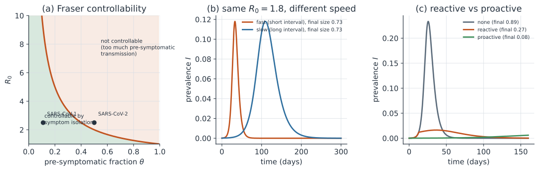
This is a boundary in the $(\theta, R_0)$ plane: below the curve $R_0 = 1/\theta$ symptom-based isolation alone can drive transmission under one, and above it the outbreak escapes no matter how fast cases are isolated. SARS-CoV-1, with modest pre-symptomatic transmission, sits in the controllable region and was contained by isolation and contact tracing; SARS-CoV-2, with roughly half of transmission occurring before symptoms, sits above the boundary, which is why symptom-based control failed and testing had to catch infections before onset.

Real isolation is imperfect, averting only a fraction $\varepsilon$ of post-symptomatic transmission. Then $R = R_0\big[\theta + (1-\theta)(1-\varepsilon)\big]$ , and setting $R = 1$ gives the critical isolation effectiveness

$\varepsilon^\ast = \frac{1 - 1/R_0}{1 - \theta} .$

When $\varepsilon^\ast > 1$ no amount of isolation suffices, which happens exactly when $\theta > 1/R_0$ .

Speed versus strength

Two interventions can leave the same number of people infected in total yet produce very different epidemics along the way (Dushoff & Park 2021, doi:10.1098/rspb.2020.1556). The strength of an intervention is the proportional reduction in transmission, which sets the effective reproduction number and therefore the final size and peak height. The speed is how fast transmission turns over, set by the generation interval, which controls the timing of the epidemic. In the middle panel two epidemics share the same $R_0$ and hence the same final size and peak prevalence, but the one with the shorter generation interval peaks months earlier. Speed matters most when generation intervals are short: a fast pathogen leaves little time to detect, decide, and deploy, so the same measure applied a week late accomplishes far less.

Control fast or control smart

Because acting early is worth more against fast pathogens, there is a value-of-information trade-off between controlling immediately and waiting to learn whether control is even needed (Thompson et al. 2018, doi:10.1371/journal.pcbi.1006014). Waiting buys information that can prevent a costly response to an outbreak that would have fizzled on its own, but for a pathogen that spreads quickly the epidemic grows during the wait, and by the time the evidence is conclusive the window for cheap control has closed. The decision therefore depends on the growth rate, the cost of acting, and how quickly surveillance resolves uncertainty, not on the final reproduction number alone.

Reactive versus proactive

The sharpest version of the timing problem is control that triggers only on detection. The right panel simulates a fast outbreak under no control, under reactive control that lowers transmission once cumulative incidence crosses a detection threshold, and under proactive control that lowers transmission from the start. Reactive control bends the curve, but because detection lags transmission it arrives after much of the spread has already happened, so it permits several times as many infections as the proactive measure. This echoes the surveillance-timing lesson from dairy-farm influenza: a detection threshold sampled too infrequently cannot keep pace with spread, so restricting introduction and transmission up front, through biosecurity, beats waiting to react.

A worked example

Take SARS-CoV-2 with $R_0 = 2.5$ and $\theta = 0.5$ : the critical isolation effectiveness is $\varepsilon^\ast = (1 - 1/2.5)/(1 - 0.5) = 1.2$ , greater than one, so isolation on symptoms cannot control it even if perfect. Take SARS-CoV-1 with the same $R_0 = 2.5$ but $\theta = 0.11$ : now $\varepsilon^\ast = (1 - 0.4)/0.89 \approx 0.67$ , so isolating about two-thirds of post-symptom transmission suffices. The same $R_0$ gives opposite control verdicts purely through the timing of infectiousness relative to symptoms.

In code

We compute the critical isolation effectiveness for several pathogens and flag which are controllable by symptom-based isolation alone.

R

critical_isolation <- function(R0, theta) (1 - 1 / R0) / (1 - theta)

pathogens <- data.frame(
  name  = c("SARS-CoV-1", "SARS-CoV-2 (ancestral)",
            "Pandemic influenza", "Smallpox"),
  R0    = c(2.5, 2.5, 1.8, 5.0),
  theta = c(0.11, 0.50, 0.45, 0.02)
)
pathogens$eps_crit     <- with(pathogens, critical_isolation(R0, theta))
$pathogens $controllable <- pathogens$ eps_crit <= 1
pathogens

Python

We use Polars to tabulate the critical isolation effectiveness.

import polars as pl

def critical_isolation(R0, theta):
    return (1 - 1 / R0) / (1 - theta)     # solves R = 1 for isolation effort

pathogens = [
    ("SARS-CoV-1", 2.5, 0.11),
    ("SARS-CoV-2 (ancestral)", 2.5, 0.50),
    ("Pandemic influenza", 1.8, 0.45),
    ("Smallpox", 5.0, 0.02),
]
rows = [{"pathogen": name, "R0": R0, "theta": theta,
         "eps_crit": round(critical_isolation(R0, theta), 3),
         "controllable": critical_isolation(R0, theta) <= 1.0}
        for name, R0, theta in pathogens]

print(pl.DataFrame(rows))

shape: (4, 5)
┌────────────────────────┬─────┬───────┬──────────┬──────────────┐
│ pathogen               ┆ R0  ┆ theta ┆ eps_crit ┆ controllable │
│ ---                    ┆ --- ┆ ---   ┆ ---      ┆ ---          │
│ str                    ┆ f64 ┆ f64   ┆ f64      ┆ bool         │
╞════════════════════════╪═════╪═══════╪══════════╪══════════════╡
│ SARS-CoV-1             ┆ 2.5 ┆ 0.11  ┆ 0.674    ┆ true         │
│ SARS-CoV-2 (ancestral) ┆ 2.5 ┆ 0.5   ┆ 1.2      ┆ false        │
│ Pandemic influenza     ┆ 1.8 ┆ 0.45  ┆ 0.808    ┆ true         │
│ Smallpox               ┆ 5.0 ┆ 0.02  ┆ 0.816    ┆ true         │
└────────────────────────┴─────┴───────┴──────────┴──────────────┘

A critical effectiveness above one means isolation on symptoms cannot hold transmission below one on its own, the situation for ancestral SARS-CoV-2 and the reason control leaned on mass testing and distancing rather than symptom-based isolation.

Julia

critical_isolation(R0, theta) = (1 - 1 / R0) / (1 - theta)

pathogens = [("SARS-CoV-1", 2.5, 0.11),
             ("SARS-CoV-2 (ancestral)", 2.5, 0.50),
             ("Pandemic influenza", 1.8, 0.45),
             ("Smallpox", 5.0, 0.02)]

for (name, R0, theta) in pathogens
    eps = critical_isolation(R0, theta)
    println((name, R0, theta, round(eps, digits = 3), eps <= 1.0))
end

Why it matters

Control is not one lever but two, and confusing them wastes effort. Strength sets how many people are ultimately infected, while speed sets how much time you have to act, and the pre-symptomatic fraction sets whether the cheapest tool, isolating the sick, can work at all. Fast pathogens with substantial pre-symptomatic transmission defeat reactive strategies because detection lags spread, which is why the effective responses to them lower introduction and transmission before cases mount rather than after. Reading an outbreak through the $(\theta, R_0)$ plane and the speed-strength decomposition turns the reproduction number and the generation interval into a concrete plan for what to deploy and how soon.