Excess Mortality

When a pandemic, heat wave, or conflict strikes, the official cause-specific death count almost always undercounts the true toll. Deaths go unattributed because testing is limited, because the crisis kills indirectly through overwhelmed health systems, and because reporting lags. Excess mortality sidesteps all of this by asking a simpler question: how many more people died than we would have expected in normal times? It is the most complete and most comparable measure of a crisis’s mortality burden.

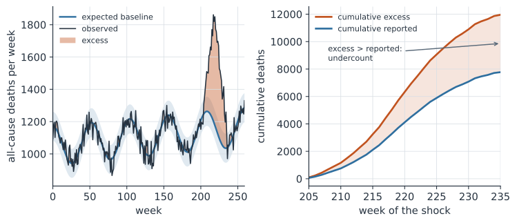
Figure 1. Left: weekly all-cause deaths with a seasonal expected baseline and prediction band, and a pandemic shock where observed deaths rise far above the baseline, with the excess shaded. Right: cumulative excess deaths running above cumulative reported cause-specific deaths, the gap being the undercount.

The idea: observed minus expected#

Excess mortality is the difference between the deaths actually observed in a period and the deaths that would have been expected absent the crisis,

$\text{excess} = \sum_t \big(O_t - E_t\big),$

where $O_t$ is observed deaths in week $t$ and $E_t$ the expected baseline. The whole problem reduces to estimating $E_t$ — a counterfactual of what mortality would have been — from the historical pattern of deaths before the crisis. Because it uses all-cause deaths, excess mortality needs no cause-of-death coding and no testing, which is exactly why it captures the deaths that a cause-specific count misses.

The expected baseline#

The classic tool is a Serfling model: a regression of weekly all-cause deaths on a slow secular trend and harmonic (sine and cosine) terms that capture the strong annual seasonality of mortality, with its winter peak (Serfling 1963). The model is fit to pre-crisis years, deliberately excluding known epidemic periods so the baseline represents normal times, then projected forward to give $E_t$ and a prediction interval during the crisis. Deaths above the upper bound of that interval are the excess. More flexible baselines — generalized linear models with overdispersion, or time-series and spline models — refine the same idea, and the choice of baseline period and model is the main source of disagreement between excess-mortality estimates.

Why it beats reported deaths#

During COVID-19, excess mortality ran well above reported COVID deaths in most countries, and the two diverged most where testing was weakest (Weinberger et al. 2020). The gap has two sources. Undercounted direct deaths are true crisis deaths never coded as such, from missed diagnoses to home deaths. Indirect deaths are the collateral toll — untreated heart attacks, deferred care, an overwhelmed hospital — that a cause-specific count would never attribute to the crisis but that excess mortality includes by construction. The same construction can produce negative excess, for instance when lockdowns cut road deaths and influenza transmission, which is a feature: excess mortality is a net measure of a crisis’s full effect on death.

A worked example#

We take observed weekly deaths over a shock period and a modeled expected baseline, sum the excess, and compare it to the deaths reported as due to the specific cause.

In code#

R#

observed <- c(1150, 1300, 1600, 1850, 1700, 1400, 1200)   # weekly deaths
expected <- c(1050, 1080, 1100, 1120, 1100, 1080, 1050)   # Serfling baseline

excess <- sum(observed - expected)
reported <- round(0.65 * excess)      # deaths coded to the specific cause
undercount_ratio <- excess / reported

round(c(excess = excess, reported = reported,
        undercount_ratio = undercount_ratio), 2)

Python#

Python

import numpy as np

observed = np.array([1150, 1300, 1600, 1850, 1700, 1400, 1200])  # weekly
expected = np.array([1050, 1080, 1100, 1120, 1100, 1080, 1050])  # baseline

excess = int((observed - expected).sum())
reported = round(0.65 * excess)        # deaths coded to the specific cause
undercount_ratio = excess / reported

print(f"excess deaths       = {excess}")
print(f"reported cause deaths = {reported}")
print(f"undercount ratio    = {undercount_ratio:.2f}")

excess deaths       = 2620
reported cause deaths = 1703
undercount ratio    = 1.54

Julia#

Julia

observed = [1150, 1300, 1600, 1850, 1700, 1400, 1200]   # weekly deaths
expected = [1050, 1080, 1100, 1120, 1100, 1080, 1050]   # Serfling baseline

excess = sum(observed .- expected)
reported = round(Int, 0.65 * excess)     # deaths coded to the specific cause
undercount_ratio = excess / reported

(excess = excess, reported = reported, undercount_ratio = undercount_ratio)

The reported cause-specific deaths capture only part of the excess; the ratio above one is the factor by which the official count understates the toll.

Why it matters#

Excess mortality is the benchmark against which every cause-specific death count is judged, because it is hard to game and easy to compare across countries with very different testing and coding practices. Its weakness is the counterfactual: the estimate is only as good as the baseline, and reasonable analysts choosing different baseline periods or models will disagree, so a credible figure reports that uncertainty. Read alongside a censoring-corrected severity estimate, excess mortality closes the loop between how many were infected, how many died, and how many of those deaths ever made it into the official record.

Severity: Estimating the CFR and IFR — the fatality ratios that reported deaths feed
Prospective Outbreak Detection — the same baseline-and-exceedance logic for detection
Surveillance Systems — the vital-registration data behind all-cause mortality
Generalized Linear Models — the regression behind the Serfling baseline
Capture-Recapture and Multiplier Methods — another route to counts the surveillance system misses