Nested Within- and Between-Host Models

The evolution of virulence rests on a trade-off between transmission and harm, but that curve is usually drawn by hand rather than derived. A nested model closes the gap: a fast within-host process sets the transmission rate $\beta$ and virulence $\alpha$ that a slow between-host SIR model treats as parameters. The trade-off then emerges from viral replication rather than being assumed, and the virulence that maximizes between-host $R_0$ is an output of the coupled system (Mideo, Alizon & Day 2008).

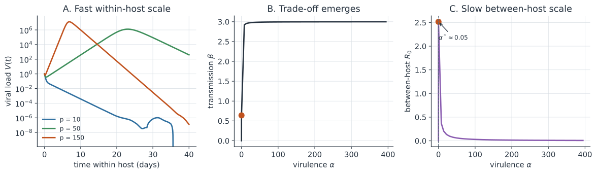
Three panels: fast within-host viral load trajectories for a sweep of replication rates, the transmission-virulence trade-off that emerges from that sweep, and the between-host basic reproduction number across virulence with the emergent optimum marked.

Two coupled scales

Infection runs on two clocks that differ by orders of magnitude in speed.

Inside one host, virus replicates over hours to days. Take a minimal target-cell model with target cells $T$ , infected cells $I$ , and free virus $V$ :

$\begin{aligned} \frac{dT}{dt} &= -b\,T V \\ \frac{dI}{dt} &= b\,T V - d\,I \\ \frac{dV}{dt} &= p\,I - c\,V. \end{aligned}$

The single parameter that a pathogen can evolve here is the virion production rate $p$ : a faster-replicating strain reaches a higher peak viral load $\bar V = \max_t V(t)$ .

Between hosts, the pathogen spreads over days to weeks in an SIR population, where the epidemiological parameters are not free constants but functions of the within-host state.

From viral load to $\beta$ and $\alpha$

The nesting is the pair of maps that turn a within-host summary into between-host rates. Transmission saturates with viral load, because a host can only shed and contact so many others, so we write an increasing, saturating map

$\beta(\bar V) = \beta_{\max}\,\frac{\bar V}{\bar V + K},$

while disease-induced mortality (virulence) climbs with the damage a high load does,

$\alpha(\bar V) = a\,\bar V.$

Both increase with $\bar V$ , so raising within-host replication $p$ raises transmission and virulence together. This shared dependence is what generates the trade-off: $\beta$ and $\alpha$ are not independent knobs but two readouts of the same underlying viral load (Gilchrist & Coombs 2006).

The emergent trade-off and its optimum

Feed the two maps into the between-host reproduction number for an SIR infection,

$R_0 = \frac{\beta(\bar V)}{\alpha(\bar V) + \gamma + \mu},$

with recovery rate $\gamma$ and background mortality $\mu$ . As $p$ sweeps from low to high, plotting $\beta$ against $\alpha$ traces out the classic trade-off curve as an output of the nested model, not an input. Because transmission saturates while virulence keeps rising, $R_0$ has an interior maximum at some finite replication rate: an emergent optimal virulence $\alpha^\*$ , exactly the singular strategy of the adaptive-dynamics analysis, now derived from mechanism.

Fitness across scales

The two scales define two different notions of fitness, and they need not agree. Within a host, selection acts on competitive success among viral variants, which favors faster replication and higher peak load. Between hosts, selection acts on $R_0$ , which is maximized at intermediate replication.

When within-host competition pushes replication past the between-host optimum, the pathogen evolves higher virulence than is best for its own spread: short-sighted evolution, where within-host wins cost between-host fitness (Gilchrist & Coombs 2006). The Price equation makes this conflict precise by partitioning selection into within- and between-host components with opposite signs.

Assumptions and caveats

The nesting buys mechanism, but it hides as much as it reveals (Handel & Rohani 2015). It assumes a clean timescale separation, so the within-host trajectory reaches its summary $\bar V$ before between-host dynamics matter. It usually assumes a single infecting strain per host, sidestepping the within-host competition that drives short-sighted evolution. And collapsing an entire viral time course to one scalar $\bar V$ discards the shape of the infectiousness profile, which itself shapes transmission. Reading across the scales is a modeling choice, not a free lunch (Mideo, Alizon & Day 2008).

A worked example

Take the within-host model with $T_0 = 10^6$ , infection rate $b = 2\times 10^{-7}$ , infected-cell death $d = 1$ , and viral clearance $c = 5$ . Sweep the replication rate $p$ from 2 to 200 and record each peak load $\bar V$ . Map load to rates with $\beta_{\max} = 3$ , $K = 10^4$ , and $a = 2\times 10^{-5}$ , and set $\gamma + \mu = 0.2$ . The between-host $R_0 = \beta/(\alpha + 0.2)$ rises, peaks, and falls; the emergent optimum sits near $\alpha^\* \approx 0.04$ , reached at a moderate replication rate well short of the fastest strain in the sweep.

In code

The executed block sweeps replication rate, integrates the within-host model for each, and reports the virulence that maximizes between-host $R_0$ .

Python

import numpy as np
from scipy.integrate import solve_ivp

# Fast within-host target-cell model: T target cells, I infected, V virus.
T0, b, dI, c = 1e6, 2e-7, 1.0, 5.0

def peak_load(p):
    def rhs(t, y):
        T, I, V = y
        return [-b * T * V, b * T * V - dI * I, p * I - c * V]
    sol = solve_ivp(rhs, [0, 40], [T0, 0.0, 1.0], method="LSODA",
                    rtol=1e-8, atol=1e-6, dense_output=True)
    t = np.linspace(0, 40, 4000)
    return sol.sol(t)[2].max()

# Map peak viral load to between-host transmission and virulence.
beta_max, Kb, a_v, d0 = 3.0, 1e4, 2e-5, 0.2   # d0 = gamma + mu
ps = np.linspace(2, 200, 60)
Vmax = np.array([peak_load(p) for p in ps])
beta = beta_max * Vmax / (Vmax + Kb)
alpha = a_v * Vmax
R0 = beta / (alpha + d0)
i = int(np.argmax(R0))
print(f"emergent optimum: alpha* = {alpha[i]:.3f}, R0 = {R0[i]:.3f}")
print(f"peaks at replication rate p = {ps[i]:.1f} (of {ps.min():.0f}-{ps.max():.0f})")

emergent optimum: alpha* = 0.039, R0 = 2.059
peaks at replication rate p = 32.2 (of 2-200)

R

library(deSolve)

T0 <- 1e6; b <- 2e-7; dI <- 1; cc <- 5
peak_load <- function(p) {
  rhs <- function(t, y, ...) {
    with(as.list(y), list(c(
      dT = -b * T * V,
      dI = b * T * V - dI * I,
      dV = p * I - cc * V)))
  }
  out <- ode(c(T = T0, I = 0, V = 1), seq(0, 40, 0.01), rhs, parms = NULL)
  max(out[, "V"])
}

beta_max <- 3; Kb <- 1e4; a_v <- 2e-5; d0 <- 0.2
ps <- seq(2, 200, length.out = 60)
Vmax <- sapply(ps, peak_load)
beta <- beta_max * Vmax / (Vmax + Kb)
alpha <- a_v * Vmax
R0 <- beta / (alpha + d0)
alpha[which.max(R0)]      # emergent optimal virulence

Julia

using DifferentialEquations

T0, b, dI, c = 1e6, 2e-7, 1.0, 5.0
function peak_load(p)
    rhs!(du, y, _, t) = begin
        T, I, V = y
        du[1] = -b * T * V
        du[2] = b * T * V - dI * I
        du[3] = p * I - c * V
    end
    sol = solve(ODEProblem(rhs!, [T0, 0.0, 1.0], (0.0, 40.0)), Rosenbrock23())
    maximum(u[3] for u in sol.u)
end

beta_max, Kb, a_v, d0 = 3.0, 1e4, 2e-5, 0.2
ps = range(2, 200, length = 60)
Vmax = peak_load.(ps)
beta = beta_max .* Vmax ./ (Vmax .+ Kb)
alpha = a_v .* Vmax
R0 = beta ./ (alpha .+ d0)
alpha[argmax(R0)]         # emergent optimal virulence

Why it matters

Nesting turns the trade-off hypothesis from an assumption into a prediction. Once $\beta$ and $\alpha$ both descend from viral load, the intermediate optimal virulence of adaptive dynamics is a theorem about the coupled system rather than a curve chosen to make the argument work. The framing also clarifies when interventions backfire: a therapy that suppresses within-host load moves the pathogen along the emergent trade-off, and a vaccine that blunts virulence without blocking transmission can select for strains that replicate harder (Mideo, Alizon & Day 2008). It is the mechanistic backbone under the population-scale story of pathogen evolution.