Transmission Tree Reconstruction (Who Infected Whom)
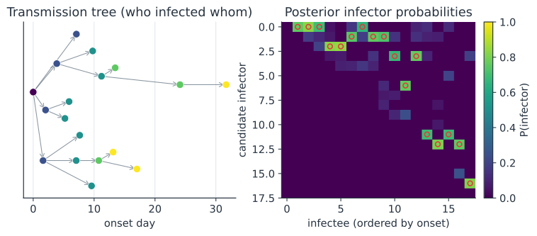
When an outbreak is over, a natural question is who infected whom. The answer — the transmission tree, naming each case’s infector — tells you where superspreading happened, whether a chain ran through a hospital or a household, and which control measures would have cut it. No single data source reveals it: case timing narrows the candidates, pathogen genomes narrow them further, and only together, run through a model, do they pin down a probable tree. This page builds a reconstruction from scratch as a runnable case study, then points to the full Bayesian tools.
Three sources of evidence#
Timing. An infector’s symptoms precede the infectee’s by roughly one serial interval — the onset-to-onset delay, whose distribution we can estimate. A case with onset today was probably infected by someone whose onset was a serial interval ago, not by someone who fell ill an hour before or a month before. This is the Wallinga-Teunis idea: score each candidate infector by the serial-interval density at the observed gap.
Genomes. A pathogen accumulates mutations as it passes from host to host, so two cases linked by direct transmission have genomes separated by only a few changes, while distantly linked cases differ more. Genetic distance discriminates among the candidates that timing alone leaves tied — but it is not the whole story, because within-host diversity and unsampled intermediates mean a small genetic distance is necessary, not sufficient, for direct transmission.
Space and contact. Who was where, and who contacted whom, sharpen the picture further; we leave them out of the case study but they enter the same way, as another factor in the infector score.
Phylogenetic tree versus transmission tree#
A common trap is to read a phylogenetic tree of the pathogen genomes as if it were the transmission tree. They are different objects. The phylogeny traces the ancestry of the sampled virus lineages; the transmission tree traces infections between hosts. They diverge because the virus diversifies within a host before onward transmission (so the lineages’ common ancestor predates the infection event), and because unsampled or missing hosts sit on transmission links that the phylogeny cannot show. Serious reconstruction models this gap explicitly rather than equating the two.
A worked case study#
We simulate an outbreak in which we know the true infector of every case, generate a genome for each case by mutating its infector’s genome, then try to recover the tree from onset times and sequences alone — exactly what we would have in a real investigation. Each code block builds on the previous one.
1. Simulate the outbreak and genomes#
import numpy as np
from scipy.stats import gamma as gamma_dist

rng = np.random.default_rng(1834)

n_cases = 40
si_mean, si_sd = 5.0, 2.0                 # serial interval (days)
si_shape = (si_mean / si_sd) ** 2
si_scale = si_sd ** 2 / si_mean
mut_per_link = 0.9                        # expected mutations per transmission
genome_len = 12000

# Build a transmission chain: case 0 is the index. Each later case is infected
# by a uniformly chosen earlier case, an onset one serial interval later.
infector = np.full(n_cases, -1)
onset = np.zeros(n_cases)
for j in range(1, n_cases):
    i = rng.integers(0, j)                # true infector, an earlier case
    infector[j] = i
    onset[j] = onset[i] + gamma_dist.rvs(si_shape, scale=si_scale,
                                         random_state=rng)

# Genomes: start from an all-zero ancestor; mutate along each transmission link.
genomes = np.zeros((n_cases, genome_len), dtype=np.int8)
for j in range(1, n_cases):
    genomes[j] = genomes[infector[j]].copy()
    n_mut = rng.poisson(mut_per_link)
    genomes[j, rng.integers(0, genome_len, n_mut)] ^= 1

print(f"simulated {n_cases} cases over {onset.max():.0f} days")
print(f"true index case: 0; example link: case 1 infected by {infector[1]}")
simulated 40 cases over 32 days
true index case: 0; example link: case 1 infected by 0
2. Score infectors by timing (Wallinga-Teunis)#
For every case we score each earlier case by the serial-interval density at the gap , then normalize into a probability distribution over candidate infectors.
def si_pdf(dt):
    return gamma_dist.pdf(dt, si_shape, scale=si_scale)

P_time = np.zeros((n_cases, n_cases))     # P_time[i, j] = P(i infected j)
for j in range(n_cases):
    for i in range(n_cases):
        dt = onset[j] - onset[i]
        if dt > 0:                        # an infector's onset precedes
            P_time[i, j] = si_pdf(dt)
    total = P_time[:, j].sum()
    if total > 0:
        P_time[:, j] /= total

ml_time = P_time[:, 1:].argmax(axis=0)    # most likely infector of cases 1..n
acc_time = np.mean(ml_time == infector[1:])
print(f"accuracy from timing alone: {acc_time:.1%}")
accuracy from timing alone: 25.6%
3. Add the genomes#
We compute the pairwise single-nucleotide distance between every pair of genomes, model the number of mutations on a direct link as Poisson with mean mut_per_link, and multiply the timing and genetic scores.
from scipy.stats import poisson

# Pairwise SNP (Hamming) distances between all genomes.
snp = (genomes[:, None, :] != genomes[None, :, :]).sum(axis=2)

def gen_lik(d):
    return poisson.pmf(d, mut_per_link)   # P(d mutations on one link)

P_comb = np.zeros((n_cases, n_cases))
for j in range(n_cases):
    for i in range(n_cases):
        dt = onset[j] - onset[i]
        if dt > 0:
            P_comb[i, j] = si_pdf(dt) * gen_lik(snp[i, j])
    total = P_comb[:, j].sum()
    if total > 0:
        P_comb[:, j] /= total

ml_comb = P_comb[:, 1:].argmax(axis=0)
acc_comb = np.mean(ml_comb == infector[1:])
print(f"accuracy from timing alone     : {acc_time:.1%}")
print(f"accuracy from timing + genomes : {acc_comb:.1%}")
accuracy from timing alone     : 25.6%
accuracy from timing + genomes : 89.7%
4. The reconstructed tree and its confidence#
We take each case’s most probable infector as the reconstructed tree, count how many links are right, and inspect where the reconstruction is confident versus uncertain.
recon = ml_comb                           # inferred infector of cases 1..n
correct = recon == infector[1:]
confidence = P_comb[recon, np.arange(1, n_cases)]   # posterior of chosen link

print(f"links recovered: {correct.sum()} of {n_cases - 1}")
print(f"mean posterior on the chosen infector: {confidence.mean():.2f}")
print("\ncase  true  inferred  P(inferred)  correct")
for j in range(1, 9):
    c = "yes" if recon[j - 1] == infector[j] else "no"
    print(f"{j:>4}  {infector[j]:>4}  {recon[j - 1]:>8}  "
          f"{P_comb[recon[j - 1], j]:>10.2f}  {c:>7}")
links recovered: 35 of 39
mean posterior on the chosen infector: 0.66

case  true  inferred  P(inferred)  correct
   1     0         0        1.00      yes
   2     0         0        1.00      yes
   3     1         1        0.39      yes
   4     0         0        0.92      yes
   5     2         2        0.56      yes
   6     1         1        0.95      yes
   7     4         4        0.36      yes
   8     0         0        0.58      yes
Adding the genomes lifts accuracy because timing alone cannot separate two candidates who fell ill at the same time, but their genetic distance to the infectee usually can. The per-link posterior is the honest output: some links are near-certain, others are a genuine toss-up, and reporting that uncertainty matters more than drawing one confident-looking tree.
From a heuristic to a full model#
The case study is a maximum-a-posteriori shortcut; production tools do three things it skips. They integrate over unsampled cases, so a link can run through a host who was never diagnosed, using the offspring and sampling distributions to infer how many are missing. They jointly model the phylogeny and the transmission tree, letting the within-host coalescent absorb the gap between the two — this is what TransPhylo does, taking a time-scaled phylogeny (typically dated in BEAST) and inferring the transmission tree on top of it (Didelot et al. 2017). And they sample whole trees rather than picking the best infector per case, so the output is a posterior distribution over transmission trees; outbreaker2 takes this route, combining genetic, temporal, and contact data in one likelihood (Campbell et al. 2018). The case study is the skeleton these put flesh on, and it is enough to see why genomes plus timing beat either alone.
The real tools in R#
In practice you would not hand-roll the estimator; outbreaker2 takes the same three evidence streams — onset dates, an alignment, and generation-time and incubation distributions — and returns a posterior over infectors.
library(outbreaker2)

# dates: onset dates; dna: an ape::DNAbin alignment (one sequence per case);
# w_dens / f_dens: discretised generation-time and incubation distributions.
data <- outbreaker_data(dates = onset_dates, dna = alignment,
                        w_dens = gen_time_pmf, f_dens = incubation_pmf)

res <- outbreaker(data = data,
                  config = create_config(n_iter = 20000, sample_every = 50))

summary(res)                              # res$alpha_* hold the sampled infectors
plot(res, type = "alpha", burnin = 2000)  # per-case infector posteriors
When you already have a time-scaled phylogeny — for example one dated in BEAST — TransPhylo infers the transmission tree on top of it, integrating over unsampled hosts and the within-host coalescent.
library(TransPhylo)

# ptree: a dated phylogeny converted with ptreeFromPhylo(); dateT: end of sampling.
res <- inferTTree(ptree, w.shape = 2, w.scale = 2.5,   # generation-time gamma
                  dateT = 2020.5)
plot(res)                                              # sampled transmission trees
medTTree(res)                                          # a point-estimate tree
Why it matters#
Reconstructing who infected whom turns a list of cases into a map of transmission, which is what reveals superspreading events, hospital or household chains, and the introductions that seeded an outbreak. The central lesson is that no single data stream suffices — timing brackets the when, genomes discriminate the who, and a model that respects both, plus the unsampled cases and the within-host gap, is what produces a defensible tree. The output worth trusting is not one tree but a distribution over trees, with a posterior on every link.
Related#
- Genomic Surveillance — the sequence data that powers reconstruction
- Phylogenetic Inference — building and dating the tree TransPhylo needs
- Phylodynamics — reading population dynamics off the same genomes
- Epidemiological Intervals and Delays — the serial interval the timing score uses
- Superspreading and Transmission Heterogeneity — what the reconstructed tree reveals about offspring variation