Pathways to Zoonotic Spillover
Most human pathogens started in animals, but a reservoir infection becomes a human case only after clearing a series of barriers, each with its own probability of being crossed. Once a pathogen does reach a person it usually spreads badly at first, producing short, mostly self-extinguishing chains of transmission, and only rarely does a lineage take off or adapt into something that transmits well. Spillover is the organizing idea behind emergence and One Health surveillance: it tells you where to watch, and it explains why counting small clusters is informative about a pathogen you cannot yet see in humans.
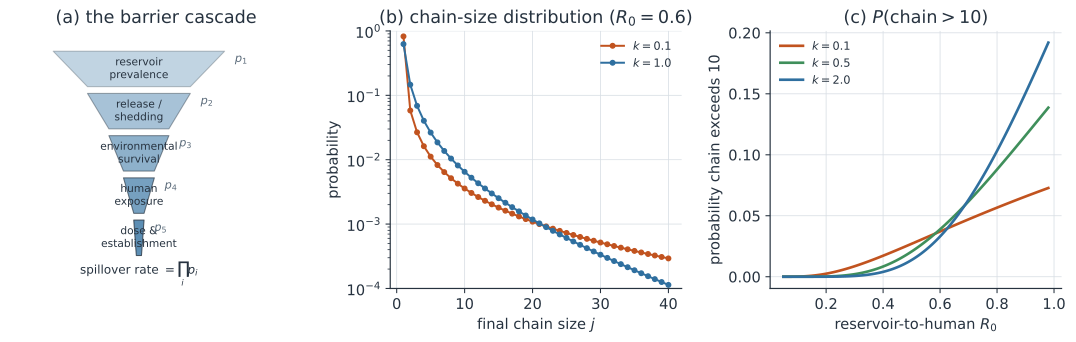
The spillover cascade#
A pathogen crosses from reservoir to human through an ordered sequence of stages. The reservoir must be infected and shedding, the pathogen must survive in the environment or vector long enough to reach a person, the person must be exposed at a sufficient dose, and the pathogen must establish within that host (Plowright et al. 2017, doi:10.1038/nrmicro.2017.45). Each stage passes only a fraction of what enters it, so if is the probability of clearing stage , the overall per-contact spillover rate is the product
Because the barriers multiply, spillover is rare even when each individual barrier is only moderately protective, and a control measure that lowers any single lowers the whole product. This is why interventions as different as vaccinating reservoir hosts, reducing human contact with wildlife, and improving reservoir ecology monitoring all act on the same funnel.
Subcritical chains#
Clearing the cascade delivers one human infection, not an epidemic. A pathogen that is poorly adapted to humans has a reproduction number below one, , so each introduction seeds a branching process that is certain to go extinct. Extinction is guaranteed, but the size of a chain before it dies is random: the final size of a chain started by one case has mean
which grows without bound as . A pathogen that almost spreads therefore produces long stuttering chains that give it many chances to adapt, the setup behind evolutionary emergence.
Individual variation and superspreading#
The mean hides how transmission is distributed across people. Real outbreaks are dominated by a few superspreaders while most cases infect no one, captured by giving the offspring count a negative binomial distribution with mean and dispersion parameter (Lloyd-Smith et al. 2005, doi:10.1038/nature04153). Small means high individual variation: the variance is , so as almost every chain dies immediately while a rare few explode. The Poisson offspring model is the limit , in which everyone transmits alike. For the same mean , smaller raises the extinction probability of a single introduction yet fattens the tail of chain sizes, so superspreading makes outbreaks simultaneously easier to contain on average and more prone to occasional large clusters.
Inferring from chains#
Because chain size depends on both and , the distribution of observed cluster sizes lets you estimate them from surveillance of stuttering transmission, without ever measuring transmission directly. For negative binomial offspring the probability that a chain reaches final size has a closed form (Blumberg & Lloyd-Smith 2013, doi:10.1371/journal.pcbi.1002993):
Fitting this to a set of observed cluster sizes returns a joint estimate of the reproduction number and the dispersion, which is how post-elimination measles clusters, monkeypox chains, and early MERS-CoV clusters were used to bound human-to-human transmission.
A worked example#
Take a spillover pathogen with and compare a superspreading strain () with a homogeneous one (). Both have the same expected chain size, cases. Under the closed-form distribution the superspreading strain produces a size-one chain (an introduction that infects no one) about of the time versus about for the homogeneous strain, yet the superspreading strain is the one that occasionally yields clusters of dozens. The same mean hides very different risks of a headline-grabbing cluster.
In code#
We simulate negative binomial branching chains at for two dispersion values and report how the chains behave.
R#
set.seed(1834)
simulate_chain <- function(R0, k, max_size = 1e4) {
  active <- 1; total <- 1
  while (active > 0 && total < max_size) {
    active <- sum(rnbinom(active, size = k, mu = R0))  # NB offspring
    total  <- total + active
  }
  total
}

R0 <- 0.6; n_chains <- 20000
for (k in c(0.1, 1.0)) {
  sizes <- replicate(n_chains, simulate_chain(R0, k))
  cat(sprintf("k=%.1f  mean=%.2f  frac>1=%.3f  frac>20=%.3f  max=%d\n",
              k, mean(sizes), mean(sizes > 1), mean(sizes > 20), max(sizes)))
}
Python#
We use Polars to hold the per-dispersion summaries.
import numpy as np
import polars as pl

rng = np.random.default_rng(1834)

def simulate_chain(R0, k, max_size=10_000):
    p = k / (k + R0)                        # NB: mean R0, dispersion k
    active, total = 1, 1
    while active > 0 and total < max_size:
        active = int(rng.negative_binomial(k, p, size=active).sum())
        total += active
    return total

R0, n_chains, threshold = 0.6, 20_000, 20
rows = []
for k in (0.1, 1.0):
    sizes = np.array([simulate_chain(R0, k) for _ in range(n_chains)])
    rows.append({"k": k, "mean_size": float(sizes.mean()),
                 "frac_gt_1": float((sizes > 1).mean()),
                 "frac_gt_20": float((sizes > threshold).mean()),
                 "max_size": int(sizes.max())})

print(pl.DataFrame(rows))
shape: (2, 5)
┌─────┬───────────┬───────────┬────────────┬──────────┐
│ k   ┆ mean_size ┆ frac_gt_1 ┆ frac_gt_20 ┆ max_size │
│ --- ┆ ---       ┆ ---       ┆ ---        ┆ ---      │
│ f64 ┆ f64       ┆ f64       ┆ f64        ┆ i64      │
╞═════╪═══════════╪═══════════╪════════════╪══════════╡
│ 0.1 ┆ 2.50285   ┆ 0.17445   ┆ 0.01935    ┆ 252      │
│ 1.0 ┆ 2.5072    ┆ 0.3776    ┆ 0.00945    ┆ 71       │
└─────┴───────────┴───────────┴────────────┴──────────┘
Both dispersion values give the same mean chain size near , but the superspreading case () leaves most introductions as isolated cases while occasionally producing a chain an order of magnitude larger than the homogeneous case ever does.
Julia#
using Distributions, Statistics, Random
Random.seed!(1834)

function simulate_chain(R0, k; max_size = 10_000)
    p = k / (k + R0)                        # NB: mean R0, dispersion k
    active, total = 1, 1
    while active > 0 && total < max_size
        active = sum(rand(NegativeBinomial(k, p), active))
        total += active
    end
    total
end

R0, n_chains = 0.6, 20_000
for k in (0.1, 1.0)
    sizes = [simulate_chain(R0, k) for _ in 1:n_chains]
    println((k = k, mean = mean(sizes), frac_gt_1 = mean(sizes .> 1),
             frac_gt_20 = mean(sizes .> 20), max = maximum(sizes)))
end
Why it matters#
Spillover turns emergence from a single frightening number into a chain of measurable probabilities, each of which is a place to intervene. The cascade explains why most pathogens never reach us and why blocking any one barrier helps; the branching-process view explains why the ones that do reach us usually fizzle; and the dispersion parameter explains why the rare exceptions can be explosive and why surveillance of small clusters is worth the effort. Reading cluster-size data through these models lets public health teams estimate how close a reservoir pathogen is to human adaptation before it ever sustains transmission, which is exactly the warning that One Health surveillance is built to provide.