Contrasts and Average Marginal Effects

A fitted logistic or Poisson model reports coefficients on the link scale — log-odds, log-rate — which are convenient to fit but awkward to communicate. An odds ratio of $1.8$ does not tell a clinician how many more infections to expect, and because these models are nonlinear, the effect of a predictor on the outcome scale depends on where every other covariate sits. Contrasts and marginal effects translate the model back onto the scale people actually act on: probability, risk, rate.

Why coefficients are not effects#

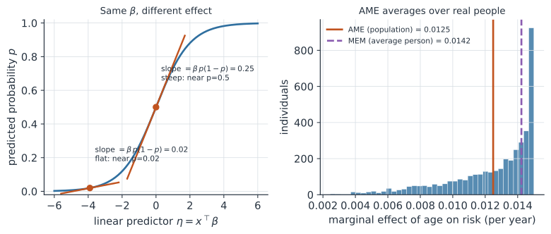
In a linear model the slope $\beta_j$ is the effect: a one-unit change in $x_j$ moves the mean by $\beta_j$ everywhere. In a nonlinear model this fails. For logistic regression the change in predicted probability from a one-unit change in $x_j$ is

$\frac{\partial p}{\partial x_j} = \beta_j \, p(1-p),$

which depends on $p$ , and therefore on every covariate through the fitted probability. The same $\beta_j$ produces a large probability change near $p = 0.5$ and almost none near $p = 0.02$ . So there is no single “effect on risk” — there is a different one for every person, and the job is to summarize them honestly.

A marginal effect#

A marginal effect is the change in the predicted outcome for a change in one predictor, holding the others fixed. For a continuous predictor it is the partial derivative above; for a categorical or binary predictor it is a contrast — a discrete difference between predictions with the variable set to two values. Because that quantity varies across the sample, you must decide where to evaluate it, and the two common choices give genuinely different numbers.

Marginal effect at the means (MEM). Set every covariate to its sample mean, then compute the effect for that one synthetic “average” person. Fast, but the average person may not exist (a mean of $0.5$ for a sex indicator describes no one).
Average marginal effect (AME). Compute the effect separately for every observed individual, using their real covariates, then average. This averages over the actual population rather than inventing a representative one, which is why it is usually the quantity you want.

The average marginal effect#

For a model with predicted mean $\hat\mu_i = g^{-1}(x_i^\top\hat\beta)$ , the AME of a continuous predictor $x_j$ is the sample mean of the individual derivatives,

$\text{AME}_j = \frac{1}{n}\sum_{i=1}^{n} \left.\frac{\partial \hat\mu_i}{\partial x_j}\right|_{x_i}.$

For a binary or categorical predictor the derivative is replaced by a difference of predictions, giving an average contrast,

$\text{AME}_j = \frac{1}{n}\sum_{i=1}^{n} \Big[\, \hat\mu_i(x_j = 1) - \hat\mu_i(x_j = 0) \,\Big],$

where every other covariate keeps its observed value and only $x_j$ is toggled. On the probability scale this average contrast is exactly a risk difference; taking the ratio of the two averaged predictions instead gives a risk ratio. This is the same computation as g-computation or standardization in causal inference: if the model is correct and confounders are included, the average contrast estimates a population-average causal effect on the natural scale.

Contrasts more generally#

A contrast is any comparison of model predictions between two settings of the covariates. That framing is more flexible than “effect of one variable”: you can contrast two specific ages, two treatment arms at a fixed age, or a whole profile against a reference. The recipe is always the same — form predictions under setting A, form them under setting B, and summarize the difference (or ratio) — which means one machinery covers risk differences, risk ratios, marginal effects, and interaction contrasts. Interactions are naturally expressed this way: the effect of treatment at age 30 versus its effect at age 70 is a contrast of contrasts, and it lives on the outcome scale where the audience can judge whether the difference matters.

Standard errors: the delta method#

A marginal effect is a nonlinear function $h(\hat\beta)$ of the estimated coefficients, so its uncertainty comes from propagating the coefficient covariance through that function. The delta method does this with a first-order Taylor expansion,

$\operatorname{Var}\!\big(h(\hat\beta)\big) \approx \nabla h(\hat\beta)^\top \, \operatorname{Var}(\hat\beta) \, \nabla h(\hat\beta),$

using the gradient of the effect with respect to the coefficients and the model’s covariance matrix $\operatorname{Var}(\hat\beta)$ . This is what marginaleffects, emmeans, and statsmodels report internally. When the effect is far from linear in $\hat\beta$ , or the sample is small, the bootstrap or simulating draws of $\hat\beta$ from its sampling distribution gives more honest intervals than the delta-method approximation.

A worked example: risk difference from a logistic model#

Here a treatment lowers infection risk, and age raises it. The logistic coefficient for treatment is a log-odds-ratio, but what a program manager wants is the average drop in probability — the average contrast, computed by predicting each person’s risk as treated and as untreated and averaging the difference.

Python

import numpy as np
import statsmodels.api as sm

rng = np.random.default_rng(42)
n = 4000
age     = rng.normal(50, 12, n)
treated = rng.binomial(1, 0.5, n)
eta = -3.0 + 0.06 * age - 0.9 * treated          # true log-odds
p   = 1 / (1 + np.exp(-eta))
y   = rng.binomial(1, p)

X   = sm.add_constant(np.column_stack([age, treated]))
fit = sm.Logit(y, X).fit(disp=False)

# odds ratio for treatment (link scale)
print(f"treatment odds ratio: {np.exp(fit.params[2]):.3f}")

# average contrast on the probability scale (g-computation):
# predict everyone as treated, then as untreated, average the difference
X1 = X.copy(); X1[:, 2] = 1.0
X0 = X.copy(); X0[:, 2] = 0.0
risk_treated   = fit.predict(X1).mean()
risk_untreated = fit.predict(X0).mean()
print(f"avg risk if treated:   {risk_treated:.4f}")
print(f"avg risk if untreated: {risk_untreated:.4f}")
print(f"average risk difference: {risk_treated - risk_untreated:.4f}")
print(f"average risk ratio:      {risk_treated / risk_untreated:.4f}")

# AME of continuous age via statsmodels' delta-method machinery
me = fit.get_margeff()                 # dydx, averaged over the sample
print(f"AME of age (per year):   {me.margeff[0]:.5f}")

treatment odds ratio: 0.374
avg risk if treated:   0.2967
avg risk if untreated: 0.5067
average risk difference: -0.2100
average risk ratio:      0.5855
AME of age (per year):   0.01213

The odds ratio is a single link-scale number, but the average risk difference and risk ratio speak directly to the outcome, and the AME of age says how many percentage points of risk each additional year of age adds on average across the real population.

In code#

R#

# marginaleffects is the standard toolkit; it handles AMEs, contrasts,
# and delta-method standard errors for almost any fitted model.
library(marginaleffects)

fit <- glm(infected ~ age + treated, data = df, family = binomial)

avg_slopes(fit)                                    # average marginal effects
avg_comparisons(fit, variables = "treated")        # average contrast (risk diff)
avg_comparisons(fit, variables = "treated",
                comparison = "ratio")              # average risk ratio

# emmeans gives the same contrasts through estimated marginal means:
library(emmeans)
emmeans(fit, ~ treated, type = "response")         # marginal risks by arm

Python#