Balanced Incomplete Block Designs

Blocking sharpens an experiment by grouping similar units, but sometimes a block is too small to hold every treatment. A taster can judge only a few wines before the palate tires; a lab technician can run only three assays in a session; a plot of land fits only a handful of varieties. A balanced incomplete block design (BIBD) chooses which treatments go in each undersized block so that, despite no block containing them all, every pair of treatments appears together equally often — which keeps all the treatment comparisons on an equal footing.

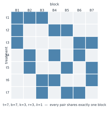
Figure 1. The (7,3,1) design as an incidence grid: 7 treatments (rows) across 7 blocks (columns), each block holding 3 treatments (filled cells). Every treatment appears in 3 blocks and every pair of treatments shares exactly one block, so no comparison is systematically better estimated than any other.

The balance conditions#

A BIBD has five parameters:

$t$ — number of treatments,
$b$ — number of blocks,
$k$ — block size (with $k < t$ , hence incomplete),
$r$ — replications of each treatment,
$\lambda$ — number of blocks in which each pair of treatments appears together.

They are not free; two identities tie them:

$b k = t r, \qquad \lambda (t - 1) = r (k - 1). \tag{1}$

The first just counts filled cells two ways. The second is the balance condition: fix a treatment, it shares its $r$ blocks with $r(k-1)$ other slots, and those must cover the remaining $t-1$ treatments exactly $\lambda$ times each ((1)). Because $\lambda$ must be a positive integer, BIBDs exist only for special parameter sets — the smallest non-trivial family being the $(t,b,k,r,\lambda) = (7,7,3,3,1)$ design shown above, whose blocks are the lines of the Fano plane.

Recovering treatment effects#

Because treatments and blocks are entangled — a treatment’s raw mean is contaminated by which blocks happened to contain it — you cannot just average. The intra-block analysis adjusts each treatment total for the blocks it fell in. With $T_i$ the total for treatment $i$ and $B_{(i)}$ the sum of totals of the blocks containing it, the adjusted treatment estimate is

$\hat{\tau}_i = \frac{k\,Q_i}{\lambda t}, \qquad Q_i = T_i - \frac{1}{k} B_{(i)}.$

The balance ( $\lambda$ constant) is exactly what makes every $\hat\tau_i$ have the same variance and every pairwise difference equally precise — the property that gives the design its name. Equivalently, fit an ordinary linear model with treatment and block factors; the least-squares treatment effects are the adjusted estimates.

A worked example#

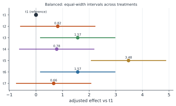
Seven diagnostic panels are compared, but each technician can validate only three per session, so the seven sessions follow the $(7,3,1)$ blocks. Each panel is run three times, and each pair of panels shares exactly one session. Simulating a response with genuine panel differences plus session-to-session shifts, and fitting a treatment-plus-block model, recovers the seven adjusted panel effects — each with the same-width interval, the hallmark of balance (Figure 2).

Figure 2. Adjusted treatment (panel) effects from the intra-block analysis, each with its 95% interval. The intervals are equal in width across treatments because every pair of treatments is compared through the same number of shared blocks — the balance the design is built to guarantee.

In code#

R#

# blocks are the (7,3,1) Fano lines; fit treatment adjusted for block
fit <- lm(y ~ factor(treatment) + factor(block), data = d)
# The treatment coefficients are the intra-block adjusted effects; because the
# design is balanced, all pairwise treatment contrasts share one variance.
library(agricolae)          # BIB.test() does the balanced analysis directly

Python#

Python

import numpy as np
import pandas as pd
import statsmodels.formula.api as smf

blocks = [(1, 2, 3), (1, 4, 5), (1, 6, 7), (2, 4, 6),
          (2, 5, 7), (3, 4, 7), (3, 5, 6)]          # (7,3,1) Fano lines
rng = np.random.default_rng(2)
tau = {t: e for t, e in zip(range(1, 8), [0, 1, 2, 1, 3, 2, 1])}
rows = []
for blk, treats in enumerate(blocks):
    shift = rng.normal(0, 2.0)                        # block (session) effect
    for t in treats:
        rows.append((t, blk, 10 + tau[t] + shift + rng.normal(0, 0.6)))
d = pd.DataFrame(rows, columns=["treatment", "block", "y"])
fit = smf.ols("y ~ C(treatment) + C(block)", data=d).fit()
adj = fit.params[[f"C(treatment)[T.{t}]" for t in range(2, 8)]]
print({f"t{t}": round(v, 2) for t, v in zip(range(2, 8), adj)})

{'t2': 0.82, 't3': 1.57, 't4': 0.78, 't5': 3.48, 't6': 1.57, 't7': 0.66}

Julia#

Julia

using DataFrames, GLM
# treatment adjusted for block gives the intra-block estimates
fit = lm(@formula(y ~ treatment + block), d, contrasts =
         Dict(:treatment => DummyCoding(), :block => DummyCoding()))

Why it matters for statistics#

Incomplete blocks are the rule, not the exception, whenever a natural grouping is small: sensory panels, split field trials, multi-reader diagnostic studies, and any experiment where fatigue, batch size, or logistics caps how many treatments a block can hold. The BIBD’s balance means that shrinking the blocks costs a little efficiency but buys equal, interpretable comparisons among all treatments — no pair is a second-class citizen. It sits alongside the Latin square as a way of removing nuisance variation by structure rather than by brute-force replication, and both are analysed through the same ANOVA partition.