Analysis of Variance
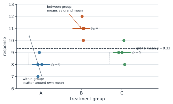
Analysis of variance answers a deceptively simple question: are these groups really different, or is the spread between their averages just the noise you would expect within any one group? The trick is to compare two kinds of variation — how far the group means sit from the grand mean, versus how much individuals scatter around their own group mean — and read off their ratio. It is the analytical engine underneath almost every designed experiment on this site, from factorial and Latin square layouts to split-plot and crossover trials.
Partitioning the variation#
Take groups with observations each, in total. Write for observation in group , for the group mean, and for the grand mean. The total spread of every point around the grand mean splits exactly into a between-group part and a within-group part:
The cross-term vanishes because deviations around each group mean sum to zero, so (1) holds identically — no approximation. SSB (between) measures the treatment signal; SSW (within) measures the residual noise.
From sums of squares to the F-ratio#
Each sum of squares carries a number of degrees of freedom: for between, for within. Dividing gives mean squares, which are variances:
If every group has the same mean, both estimate the same error variance and their ratio hovers near one. If the groups genuinely differ, SSB inflates and the ratio grows:
Under the null hypothesis of equal means (with independent, roughly normal errors of constant variance), follows an distribution, which is what turns the ratio into a p-value.
A worked example#
Three antibiotic regimens are each tried on four bacterial cultures; the response is log-reduction in colony count.
| Regimen | Values | Mean |
|---|---|---|
| A | 8, 9, 7, 8 | 8 |
| B | 10, 11, 12, 11 | 11 |
| C | 9, 8, 10, 9 | 9 |
The grand mean is . The between-group sum of squares is
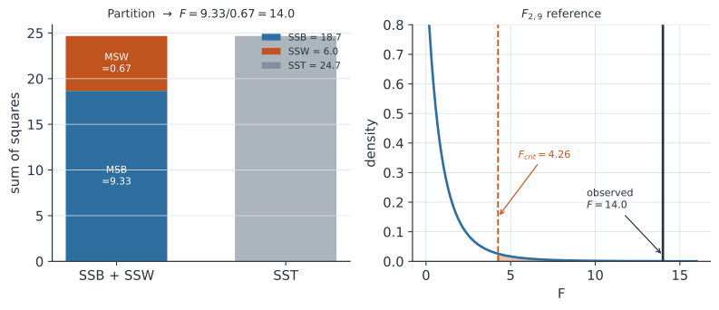
and, adding the squared deviations inside each group (),
With and degrees of freedom, and , so
Against the reference (5% critical value ) this is far into the tail — the regimens differ (Figure 2).
In code#
R#
d <- data.frame(
  y = c(8, 9, 7, 8, 10, 11, 12, 11, 9, 8, 10, 9),
  g = rep(c("A", "B", "C"), each = 4)
)
summary(aov(y ~ g, data = d))
#             Df Sum Sq Mean Sq F value  Pr(>F)
# g            2  18.67   9.333    14.0 0.00171 **
# Residuals    9   6.00   0.667
Python#
import numpy as np
from scipy import stats

groups = {
    "A": [8, 9, 7, 8],
    "B": [10, 11, 12, 11],
    "C": [9, 8, 10, 9],
}
y = np.array([v for vs in groups.values() for v in vs], float)
grand = y.mean()
ssb = sum(len(v) * (np.mean(v) - grand) ** 2 for v in groups.values())
ssw = sum(((np.array(v) - np.mean(v)) ** 2).sum() for v in groups.values())
k, N = len(groups), y.size
F = (ssb / (k - 1)) / (ssw / (N - k))
p = stats.f.sf(F, k - 1, N - k)
print(f"SSB={ssb:.2f} SSW={ssw:.2f} F={F:.2f} p={p:.4f}")
SSB=18.67 SSW=6.00 F=14.00 p=0.0017
Julia#
using Statistics, Distributions
groups = Dict("A"=>[8,9,7,8], "B"=>[10,11,12,11], "C"=>[9,8,10,9])
y = reduce(vcat, values(groups))
grand = mean(y)
ssb = sum(length(v) * (mean(v) - grand)^2 for v in values(groups))
ssw = sum(sum((v .- mean(v)).^2) for v in values(groups))
k, N = length(groups), length(y)
F = (ssb / (k - 1)) / (ssw / (N - k))
p = ccdf(FDist(k - 1, N - k), F)
println("F=$(round(F, digits=2)) p=$(round(p, digits=4))")
Why it matters for statistics#
ANOVA is the bridge between experimental design and inference: the way a study is blocked, crossed, or nested determines exactly how the total variation is carved up, and each design in this section is really a different recipe for the sum-of-squares partition. A Latin square peels off two blocking directions before testing treatments; a split-plot design produces two error strata, so the whole-plot and sub-plot factors are tested against different denominators; a repeated-measures analysis pulls out a subject term to sharpen within-subject comparisons. Understanding the partition is what lets you build the right -test — and spot when a naïve one uses the wrong error term.