Latin Square Designs
A Latin square controls two sources of nuisance variation at the same time. Where a randomized block design blocks on one factor (say technician), a Latin square blocks on two (technician and day), by arranging treatments in a grid so that each treatment appears exactly once in every row and every column. Both blocking directions are swept out of the error term, so the treatment comparison is made against unusually clean residual variation — for the cost of only runs.
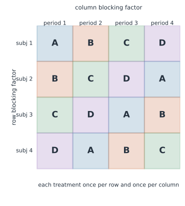
Two blocking directions#
Label the response in row , column by the treatment that sits there:
with the row effect, the column effect, and the treatment effect. The Latin-square constraint — each treatment once per row and once per column — makes the row, column, and treatment contrasts mutually orthogonal, so their effects can be estimated independently and the ANOVA sum of squares splits cleanly four ways:
The treatment effect is tested against , which now excludes both nuisance directions — the source of the design’s efficiency.
The degrees-of-freedom cost#
Orthogonality is not free. A square has observations, and the degrees of freedom go: each to rows, columns, and treatments, leaving only
for error. For that is just — thin. Small squares are therefore often replicated (several squares, or the same square rerun) to build up error degrees of freedom, and the design assumes no interactions among rows, columns, and treatments, since there is no room to estimate them.
Do not confuse this with Latin hypercube sampling, a space-filling design for computer experiments. They share the “once per row and column” Latin-square idea but solve different problems — physical blocking here, high-dimensional coverage there.
A worked example#
Four treatments A–D are given to four subjects (rows) across four periods (columns), one treatment per subject-period, arranged as a cyclic Latin square so no subject repeats a treatment and no period does either.
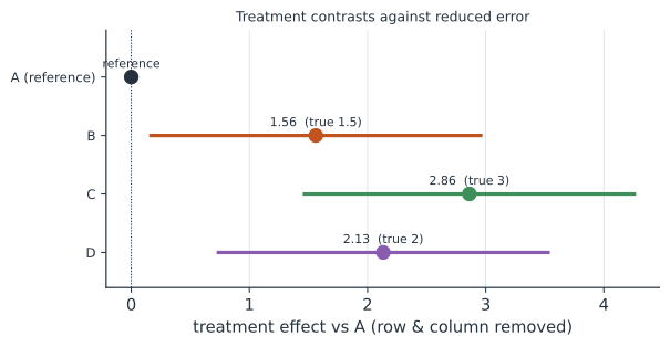
Simulating a response with real subject and period differences on top of treatment effects, then fitting y ~ row + column + treatment, partitions the variation and isolates the treatment effects — the row and column sums of squares are removed before the treatment -test, and the estimated treatment contrasts come out against the reduced error (Figure 2).
In code#
R#
# rows, columns, and treatment each enter as factors; the design's orthogonality
# makes the ANOVA partition clean
fit <- aov(y ~ factor(row) + factor(col) + treatment, data = d)
summary(fit)   # row and column SS are removed before the treatment F-test
Python#
import numpy as np
import pandas as pd
import statsmodels.formula.api as smf
from statsmodels.stats.anova import anova_lm

letters = ["A", "B", "C", "D"]
square = [[letters[(j + i) % 4] for j in range(4)] for i in range(4)]  # cyclic
rng = np.random.default_rng(4)
row_eff = rng.normal(0, 2.0, 4)                    # subject differences
col_eff = rng.normal(0, 1.5, 4)                    # period differences
tau = {"A": 0.0, "B": 1.5, "C": 3.0, "D": 2.0}
rows = []
for i in range(4):
    for j in range(4):
        t = square[i][j]
        y = 20 + row_eff[i] + col_eff[j] + tau[t] + rng.normal(0, 0.6)
        rows.append((i, j, t, y))
d = pd.DataFrame(rows, columns=["row", "col", "treatment", "y"])
fit = smf.ols("y ~ C(row) + C(col) + treatment", data=d).fit()
print(anova_lm(fit).round(2)[["df", "sum_sq", "F"]])
            df  sum_sq      F
C(row)     3.0   40.08  20.54
C(col)     3.0   32.63  16.73
treatment  3.0   17.72   9.08
Residual   6.0    3.90    NaN
Julia#
using DataFrames, GLM
# row, column, and treatment factors; orthogonal by construction
fit = lm(@formula(y ~ row + col + treatment), d, contrasts =
         Dict(:row => DummyCoding(), :col => DummyCoding()))
Why it matters for statistics#
Latin squares are the natural design whenever two nuisance factors act at once and roughly independently: field trials with fertility gradients in two directions, crossover trials where subjects and periods both matter, laboratory studies spanning several machines and several days. By balancing treatments against both directions, they extract a clean treatment comparison from a small, structured experiment — the same “remove variation by design” philosophy as the balanced incomplete block design, extended to a second blocking axis. Their limitation, the no-interaction assumption and the thin error, is the price of squeezing two-way control out of only runs.