Chain-Binomial Models and the Household Secondary Attack Rate
Households are the natural laboratory of transmission: a small, closed group with intense contact, where you can watch who infects whom over a few generations. The chain-binomial model, in its classic Reed-Frost form, is the stochastic model built for exactly this setting, and the secondary attack rate it gives rise to is the standard summary of how readily a pathogen spreads among close contacts. Together they turn a household outbreak into an estimate of transmissibility.
The Reed-Frost model#
Consider a closed group — a household of people — evolving in discrete generations. Let be the probability that a given infectious person transmits to a given susceptible during one generation, and the probability they do not. A susceptible escapes infection in a generation only by escaping every current infective independently, which happens with probability when there are infectives. So the number of new infections in the next generation is binomial,
and the susceptibles are depleted, . The chain of binomial draws — one per generation until no infectives remain — is what gives the model its name. It is the small-population, discrete-generation cousin of the branching process: the same offspring-by-chance logic, but with a finite susceptible pool that gets used up.
Household final size#
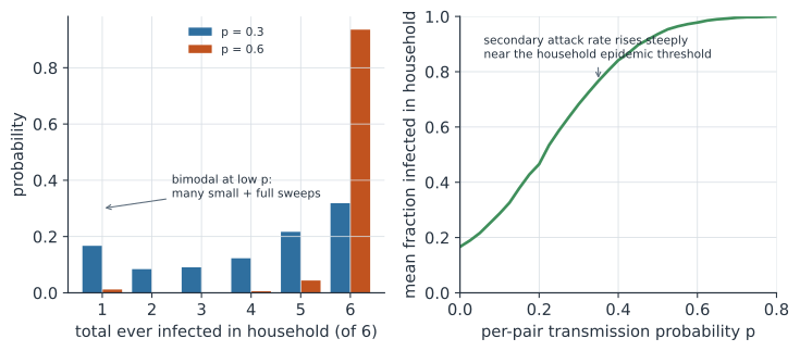
Because transmission is stochastic, a household outbreak does not have a single outcome but a distribution of final sizes — the total ever infected, from just the introducer up to the whole household. The shape of that distribution is informative. At intermediate transmission probability it is bimodal, as the left panel of the figure shows: many introductions infect only one or two people and fizzle, while a substantial minority sweep through everyone. This is the household-scale echo of the extinction-versus-invasion dichotomy, and it is why single households give noisy estimates while the distribution of final sizes across many households is highly informative — the basis of the Longini and Koopman (1982) method for estimating transmission parameters from household data.
The secondary attack rate#
The secondary attack rate (SAR) is the workhorse summary: the probability that an infectious person transmits to a given susceptible household contact over the course of the outbreak. Empirically it is estimated as
the fraction of exposed contacts who become infected, excluding the introducing case. The SAR is one of the first numbers reported for a new pathogen because household studies can be stood up quickly, and it feeds directly into transmission models and into policy on household quarantine and prophylaxis. It also cleanly separates transmissibility from exposure: everyone in a household is heavily exposed, so a low SAR reflects the pathogen, not a lack of contact — a study-design virtue shared with the test-negative design.
A worked example#
We simulate the Reed-Frost process in a household of six with one introducing case and a per-pair transmission probability of 0.4, then read off the mean final size and the secondary attack rate among the five susceptible contacts.
In code#
R#
set.seed(1834)
reed_frost <- function(n, p, reps) {
  q <- 1 - p
  replicate(reps, {
    S <- n - 1; I <- 1; total <- 1
    while (I > 0) {
      newI <- rbinom(1, S, 1 - q^I)
      S <- S - newI; total <- total + newI; I <- newI
    }
    total
  })
}

totals <- reed_frost(6, 0.4, 20000)
mean_total <- mean(totals)
sar <- (mean_total - 1) / (6 - 1)      # secondary cases / susceptibles
round(c(mean_final_size = mean_total, SAR = sar), 3)
Python#
import numpy as np

rng = np.random.default_rng(1834)

def reed_frost(n, p, reps):
    q = 1 - p
    totals = np.empty(reps, dtype=int)
    for r in range(reps):
        S, I, total = n - 1, 1, 1
        while I > 0:
            new_I = rng.binomial(S, 1 - q ** I)
            S -= new_I; total += new_I; I = new_I
        totals[r] = total
    return totals

totals = reed_frost(6, 0.4, 20000)
mean_total = totals.mean()
sar = (mean_total - 1) / (6 - 1)       # secondary cases / susceptibles

print(f"mean final size      = {mean_total:.3f}")
print(f"secondary attack rate = {sar:.3f}")
mean final size      = 5.046
secondary attack rate = 0.809
Julia#
using Random, Distributions, Statistics

Random.seed!(1834)

function reed_frost(n, p, reps)
    q = 1 - p
    totals = Vector{Int}(undef, reps)
    for r in 1:reps
        S, I, total = n - 1, 1, 1
        while I > 0
            new_I = rand(Binomial(S, 1 - q^I))
            S -= new_I; total += new_I; I = new_I
        end
        totals[r] = total
    end
    totals
end

totals = reed_frost(6, 0.4, 20000)
mean_total = mean(totals)
sar = (mean_total - 1) / (6 - 1)
(mean_final_size = mean_total, SAR = sar)
Why it matters#
The chain-binomial model is the simplest honest model of transmission in a small group, and it makes explicit that a household outbreak is a random process whose distribution of outcomes, not any single household, carries the information. The secondary attack rate it underpins is among the fastest transmissibility measures to obtain for an emerging pathogen and one of the cleanest, because heavy shared exposure lets it isolate the pathogen’s infectiousness. The bimodal final-size distribution is a reminder that with small numbers, chance dominates, and that estimates must be pooled across many households to be stable.
Related#
- Branching Processes — the large-population limit of the same offspring logic
- The Binomial Distribution — the draw at the heart of each generation
- Stochastic Epidemics and the Gillespie Algorithm — continuous-time stochastic transmission
- Superspreading and Transmission Heterogeneity — variation in how many each case infects
- Final Size, Herd Immunity, and Overshoot — final size in the large-population deterministic limit