Clustering and Unsupervised Learning
Sometimes there are no labels, only data, and the question is what structure hides inside it: which patients share a phenotype, which pathogen isolates form a lineage, which places behave alike. Clustering answers by grouping observations so that members of a group resemble each other more than they resemble members of other groups — the most-used form of unsupervised learning, alongside the dimensionality reduction of the previous page. The catch, which runs through the whole topic, is that clustering will always return groups whether or not any real ones exist, so the algorithms are the easy part and judging whether the clusters mean anything is the hard part.
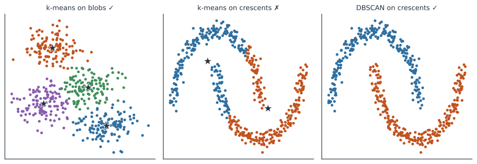
k-means#
k-means is the workhorse: choose a number of clusters , and partition the data to minimize the total within-cluster variance — the summed squared distance of each point to its cluster’s mean (centroid). Lloyd’s algorithm alternates two cheap steps until nothing moves: assign each point to its nearest centroid, then recompute each centroid as the mean of its assigned points. It is fast and scales well, but it has strong assumptions baked in: it favors spherical, equally-sized clusters, because “nearest centroid” carves space into straight-edged (Voronoi) cells — which is exactly why it splits the crescents in the middle of the figure clean in half. It also needs chosen in advance and is sensitive to the initial centroids, so the k-means++ initialization (spreading initial centroids apart) and several restarts are standard.
Gaussian mixtures and hierarchical clustering#
Two classical alternatives relax k-means’ rigidity. A Gaussian mixture model (GMM) treats the data as drawn from a mixture of Gaussian blobs and fits them by the expectation–maximization algorithm; because each cluster has its own covariance, GMMs capture elliptical clusters of different sizes, and they give soft assignments — a probability of belonging to each cluster rather than a hard label — which is often what you want when membership is genuinely uncertain. Hierarchical (agglomerative) clustering takes a different tack: start with every point its own cluster and repeatedly merge the two closest, building a dendrogram — a tree of nested groupings — that you cut at whatever level gives the number of clusters you want. It needs no up front and its tree is interpretable, which is why it is a staple for gene-expression heatmaps and for grouping pathogen isolates by genetic distance.
Density-based clustering#
DBSCAN abandons centroids entirely and defines a cluster as a connected region of high density: points with enough neighbors within a radius are “core” points, clusters grow by chaining core points together, and points in sparse regions are labeled noise rather than forced into a cluster. This buys two things k-means cannot offer. It finds clusters of arbitrary shape — the crescents on the right of the figure — because it follows density rather than distance to a center, and it needs no , discovering the number of clusters from the data. It also handles outliers gracefully by design, which makes it and its hierarchical successor HDBSCAN natural fits for spatial data and for anomaly-aware settings, complementing the reconstruction-error anomaly detection of a VAE. The price is two parameters (the radius and the minimum neighbor count) and difficulty when clusters have very different densities.
Choosing k and validating clusters#
The deepest problem is not which algorithm but whether the clusters are real. Because any method returns groups, you need to (1) choose the number of clusters and (2) sanity-check that they reflect structure, not noise. Internal measures help with both: the silhouette score rates how well each point sits in its cluster versus the next-nearest, the elbow method looks for the past which within-cluster variance stops dropping sharply, and the gap statistic compares your clustering against what you would get on featureless random data. When labels are available for validation, the adjusted Rand index measures agreement between the clustering and the truth, correcting for chance. None of these is definitive — clusters that are statistically clean may be biologically meaningless and vice versa — so cluster labels are best treated as hypotheses to be checked against external information, never as discovered facts.
A worked example#
Run one k-means iteration on six points in 1D at positions with and initial centroids at and . Assign: points are nearer , and nearer , so the two clusters are and . Update: the new centroids are the cluster means, and — unchanged, so the algorithm has already converged, with a clean split. Move one point, say a , and it joins the left cluster, dragging its centroid to ; the tug-of-war between assignment and update is all k-means ever does, and its reliance on those means is exactly why non-spherical shapes defeat it.
In code#
Python#
Which algorithm to reach for depends on the shape of the clusters — k-means recovers blobs but fails on crescents, where DBSCAN succeeds:
import numpy as np
from sklearn.datasets import make_blobs, make_moons
from sklearn.cluster import KMeans, DBSCAN
from sklearn.metrics import adjusted_rand_score, silhouette_score

Xb, yb = make_blobs(n_samples=600, centers=4, cluster_std=0.9, random_state=0)
km = KMeans(n_clusters=4, n_init=10, random_state=0).fit(Xb)
print(f"k-means on blobs:  ARI {adjusted_rand_score(yb, km.labels_):.2f}, "
      f"silhouette {silhouette_score(Xb, km.labels_):.2f}")

Xm, ym = make_moons(n_samples=600, noise=0.06, random_state=0)   # non-convex shapes
km_m = KMeans(n_clusters=2, n_init=10, random_state=0).fit(Xm)
db = DBSCAN(eps=0.20, min_samples=5).fit(Xm)
print(f"two crescents:     k-means ARI {adjusted_rand_score(ym, km_m.labels_):.2f}, "
      f"DBSCAN ARI {adjusted_rand_score(ym, db.labels_):.2f}")
k-means on blobs:  ARI 0.91, silhouette 0.54
two crescents:     k-means ARI 0.26, DBSCAN ARI 1.00
HDBSCAN is the robust modern default for density clustering — no radius to tune, and it recovers the crescents from the data alone:
import hdbscan
labels = hdbscan.HDBSCAN(min_cluster_size=15).fit_predict(Xm)   # -1 marks noise
n_found = len(set(labels)) - (1 if -1 in labels else 0)
print(f"HDBSCAN found {n_found} clusters (no k given), "
      f"ARI {adjusted_rand_score(ym, labels):.2f}")
HDBSCAN found 2 clusters (no k given), ARI 1.00
R#
# stats::kmeans / hclust; mclust for GMMs; dbscan for density clustering.
km <- kmeans(X, centers = 4, nstart = 10)
hc <- hclust(dist(X), method = "ward.D2")   # dendrogram; cut with cutree()
library(dbscan)
db <- dbscan(X, eps = 0.2, minPts = 5)
Julia#
# Clustering.jl provides kmeans, hierarchical clustering, and dbscan.
using Clustering
km = kmeans(X', 4)                  # columns are observations
db = dbscan(X', 0.2; min_neighbors = 5)
Why it matters#
Unsupervised clustering is how discovery often begins when the categories are not yet known. In genomics it groups pathogen isolates into lineages and transmission clusters and cells into types; in clinical data it defines phenotypes — subgroups of patients who share a disease pattern and may need different care; in surveillance it flags space–time clusters of cases (a data-driven complement to the model-based spatial scan statistic); and in immunology it gates cytometry populations. The recurring caution is the one this page opened with: an algorithm will always draw boundaries, so the real work is validation — checking that a cluster is stable, separates on measures the algorithm did not optimize, and corresponds to something outside the data — before a discovered “subtype” is allowed to change a decision.