Social Contact Matrices and Age-Structured Mixing

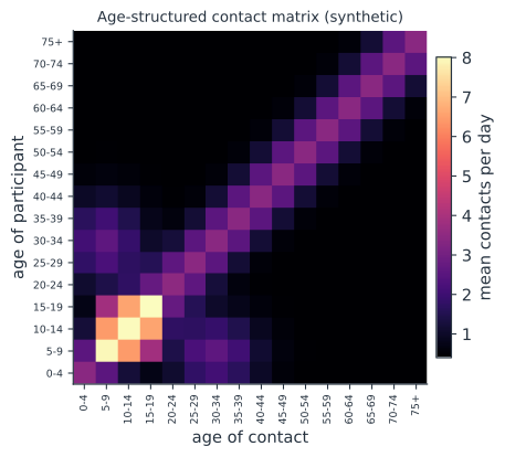
A directly transmitted pathogen spreads through the contacts people actually have, and those contacts are strongly patterned by age: children mix intensely with other children, parents with young children, and the elderly largely with each other. An age-structured transmission model needs to encode that pattern, and the object that does so is the contact matrix, whose entry in row $i$ , column $j$ is the mean number of contacts a person in age group $i$ has with people in age group $j$ per day. For a generation, modelers guessed these mixing patterns; contact surveys replaced the guesswork with measurement.

Figure 1. A synthetic age-structured social contact matrix over sixteen five-year age bands, showing a strong assortative diagonal, an intense school-age block among children and teenagers, and off-diagonal parent-child ridges linking adults in their late twenties to thirties with young children.

From WAIFW to measured contacts#

The classical approach parameterized a who-acquires-infection-from-whom (WAIFW) matrix, imposing a handful of mixing structures with names like “assortative” or “proportionate” and fitting the free parameters to serological data. The trouble is that estimates of $R_0$ turned out to be sensitive to which structure you assumed, and the choice was largely arbitrary (Goeyvaerts et al. 2010, doi:10.1111/j.1467-9876.2009.00693.x). The alternative, now standard, is to measure contact rates directly from diary-based surveys and assume transmission is proportional to contact. The POLYMOD study, in which thousands of participants across eight European countries recorded every conversational and physical contact for a day, is the canonical source and revealed the strong age assortativity and parent-child structure visible in the figure (Mossong et al. 2008, doi:10.1371/journal.pmed.0050074).

The reciprocity constraint#

Contacts are symmetric events: if a person in group $i$ meets a person in group $j$ , that is simultaneously a contact of $j$ with $i$ . At the population level this forces a reciprocity constraint on the total number of contacts,

$c_{ij}\, N_i = c_{ji}\, N_j,$

where $c_{ij}$ is the per-capita contact rate and $N_i$ the size of group $i$ . Raw survey matrices never satisfy this exactly because of sampling noise and differential reporting, so estimated matrices are symmetrized against the age distribution before use. This is why a contact matrix is inseparable from the demography of the population it describes, and why matrices measured in one country cannot be transplanted to another with a very different age structure — a live gap for much of sub-Saharan Africa, where empirical matrices remain scarce (Fung et al. 2024, doi:10.1111/tmi.14063).

From contact matrix to R₀#

The contact matrix enters transmission dynamics through the force of infection. Under the proportionality assumption, the rate at which susceptibles in group $i$ are infected is $\lambda_i = q \sum_j c_{ij} \frac{I_j}{N_j}$ , where $q$ is a per-contact transmission probability. Collecting the pieces gives a next-generation matrix whose entry is the expected number of new infections in group $i$ from one infectious individual in group $j$ ,

$K_{ij} = q\, c_{ij}\, \frac{N_i}{N_j}\, D,$

with $D$ the mean infectious period. As on the next-generation matrix page, $R_0$ is then the dominant eigenvalue (spectral radius) of $K$ , not any single entry. The age structure of the contact matrix therefore controls not just $R_0$ but who drives transmission, which is exactly the information needed to target vaccination or school-based interventions.

A worked example#

Take three age groups — children, adults, elderly — with a contact matrix that is strongly assortative, a per-contact transmission probability $q = 0.05$ , and a mean infectious period of $D = 4$ days. We build the next-generation matrix and read $R_0$ off its dominant eigenvalue.

In code#

R#

C <- matrix(c(8, 4, 1,
              4, 6, 2,
              1, 2, 3), nrow = 3, byrow = TRUE)   # contacts/day by age
N <- c(2000, 5000, 1500)                          # group sizes
q <- 0.05; D <- 4

K <- q * D * C * outer(N, N, "/")   # K_ij = q D c_ij N_i / N_j
R0 <- max(abs(eigen(K)$values))

round(R0, 3)

Python#

Python

import numpy as np

C = np.array([[8, 4, 1],
              [4, 6, 2],
              [1, 2, 3]], dtype=float)   # contacts/day by age group
N = np.array([2000, 5000, 1500], dtype=float)
q, D = 0.05, 4

K = q * D * C * (N[:, None] / N[None, :])   # K_ij = q D c_ij N_i / N_j
R0 = np.abs(np.linalg.eigvals(K)).max()

print(f"R0 = dominant eigenvalue of K = {R0:.3f}")

R0 = dominant eigenvalue of K = 2.321

Julia#

Julia

using LinearAlgebra

C = [8.0 4 1; 4 6 2; 1 2 3]    # contacts/day by age group
N = [2000.0, 5000, 1500]
q, D = 0.05, 4

K = q * D .* C .* (N * (1 ./ N)')   # K_ij = q D c_ij N_i / N_j
R0 = maximum(abs.(eigvals(K)))

round(R0; digits = 3)

Why it matters#

The contact matrix is where the social structure of a population enters an epidemic model, and getting it from measurement rather than assumption changed how reliably models estimate age-specific transmission. Because the matrix is tied to demography through reciprocity, it explains why the same pathogen produces different age patterns in different countries, and why interventions aimed at high-contact groups such as schoolchildren can have leverage out of proportion to their share of the population. It is also the bridge between the human, measurable side of transmission and the next-generation matrix machinery that turns mixing into $R_0$ .

The Next-Generation Matrix and R₀ — turning mixing into a reproduction number
SEIR and Compartmental Extensions — where age structure enters the dynamics
Density- and Frequency-Dependent Transmission — how contact scales with population
Structured Populations — matrix models across groups
Social and Structural Drivers of Transmission — who mixes with whom, and why