Hidden Markov Models

Some of the most useful hidden states are not numbers but regimes: a person is in a high-risk or a low-risk period, an epidemic is growing or declining, a stretch of genome is coding or non-coding, an animal is foraging or resting. A hidden Markov model (HMM) is the tool for exactly this — a discrete latent state that jumps between a few categories as a Markov chain, which we never observe directly but only through a noisy, state-dependent emission. It is the discrete-state sibling of the Kalman filter and the particle filter: the same predict-then-correct logic, but the belief is a small vector of category probabilities instead of a Gaussian or a particle cloud, which makes everything exact and cheap.

Consider a sexually transmitted infection with reinfection. An individual’s underlying risk regime drifts over time — a high-risk period (a new partnership, a partner with other partners) raises the monthly chance of acquiring or reacquiring infection; a low-risk period lowers it. We do not see the regime; we see a longitudinal string of test results. An HMM reconstructs the hidden risk trajectory from those tests, and estimates how sticky each regime is and how differently they generate infections.

Figure 1. Top: one person’s monthly test results, with positive tests clustering inside the true (shaded) high-risk periods. Bottom: the HMM posterior probability of being high-risk and the Viterbi most-likely regime path, both recovering the shaded episodes from the tests alone.

The model#

An HMM has three pieces. A hidden state $z_t \in \{1, \dots, K\}$ follows a Markov chain with a $K\times K$ transition matrix $A$ , where $A_{ij} = \Pr(z_t = j \mid z_{t-1} = i)$ , started from an initial distribution $\pi$ . Each state emits an observation through its own emission distribution $b_j(y_t) = \Pr(y_t \mid z_t = j)$ — here a Bernoulli, “test positive with probability $p_j$ ”, with $p_{\text{high}} \gg p_{\text{low}}$ . The Markov chain is on the hidden state, not the data: the observations are conditionally independent given the states, and all the memory lives in $z_t$ .

The likelihood of a whole series sums over every possible hidden path,

$\Pr(y_{1:T}) = \sum_{z_{1:T}} \pi_{z_1} b_{z_1}(y_1) \prod_{t=2}^{T} A_{z_{t-1} z_t}\, b_{z_t}(y_t), \tag{1}$

which has $K^T$ terms — astronomically many — yet the special Markov structure collapses it to a linear-time recursion.

Three questions, three algorithms#

Every HMM task is one of three classic problems (Rabiner 1989).

Likelihood — the forward algorithm. Define $\alpha_t(j) = \Pr(y_{1:t}, z_t = j)$ , the joint probability of the data so far and being in state $j$ now. It obeys a one-step recursion that carries the sum in (1) forward in linear time,

$\alpha_t(j) = b_j(y_t) \sum_{i=1}^{K} \alpha_{t-1}(i)\, A_{ij}, \tag{2}$

and $\Pr(y_{1:T}) = \sum_j \alpha_T(j)$ . This is the exact analogue of the Kalman filter’s predict ( $\sum_i \alpha_{t-1}(i) A_{ij}$ ) and update ( $\times\, b_j(y_t)$ ) steps.

Decoding — Viterbi and forward–backward. To recover the hidden regimes there are two answers. The Viterbi algorithm replaces the sum in (2) with a max, tracing the single most likely path $\hat{z}_{1:T}$ through the states,

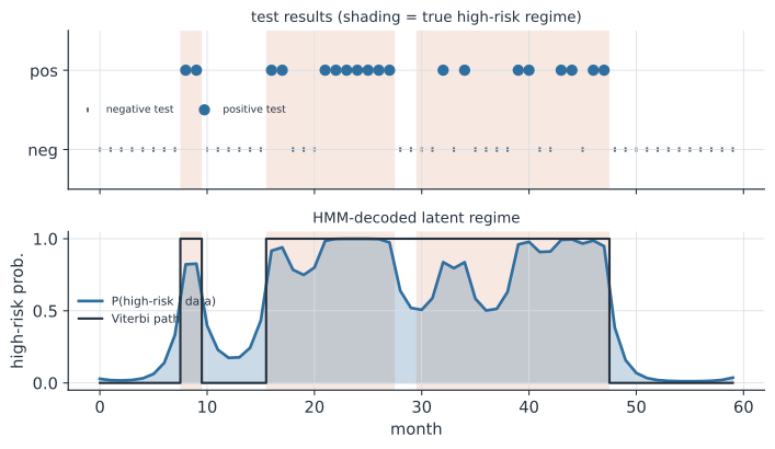
$\delta_t(j) = b_j(y_t)\, \max_i\, \delta_{t-1}(i)\, A_{ij}, \tag{3}$

with back-pointers to reconstruct the path. The forward–backward algorithm instead adds a backward pass $\beta_t$ and returns the smoothed posterior $\gamma_t(j) = \Pr(z_t = j \mid y_{1:T})$ at every step — the soft, per-time probability of each regime (the blue curve in the figure), as opposed to Viterbi’s single hard path (the dark step).

Learning — Baum–Welch. When $A$ , the emission parameters, and $\pi$ are unknown, Baum–Welch — the EM algorithm for HMMs — estimates them from the observations alone. It alternates a forward–backward pass (the E-step, computing expected state and transition counts $\gamma_t$ and $\xi_t$ ) with a re-estimation of the parameters from those expected counts (the M-step), climbing the likelihood to a local maximum. Pooling many individuals’ series sharpens the estimates enormously, which is why cohort data are ideal.

A worked example#

We simulate a cohort of 80 people, each tested monthly for five years, with a sticky low/high-risk latent regime (high-risk months are positive with probability $0.55$ , low-risk with $0.03$ ). From the test results alone — never the true regime — Baum–Welch recovers the emission and transition parameters, and Viterbi decodes each person’s hidden risk trajectory.

In code#

The R version uses depmixS4 (a standard package for latent-regime models; HMM and hmmTMB are alternatives). The Python and Julia versions implement the forward–backward, Baum–Welch, and Viterbi recursions by hand to expose the machinery.

R#

library(depmixS4)
# `tests`: long format, one row per person-month, `positive` in {0, 1}
mod <- depmix(positive ~ 1, data = tests, nstates = 2,
              family = binomial(), ntimes = rep(60, 80))   # 80 people x 60 months
set.seed(1)
fit <- fit(mod)              # Baum-Welch (EM)
summary(fit)                 # emission probabilities + transition matrix

post <- posterior(fit)       # Viterbi path (post$state) + smoothed P(state | data)

Python#

Python

import numpy as np

rng = np.random.default_rng(2)
A = np.array([[0.95, 0.05], [0.15, 0.85]])       # true low/high-risk transitions
p_inf = np.array([0.03, 0.55])                    # test-positive prob by regime
pi = np.array([0.85, 0.15])
Npat, T = 80, 60

def simulate():
    z = np.zeros(T, int); z[0] = rng.random() > pi[0]
    for t in range(1, T):
        z[t] = rng.random() > A[z[t - 1], 0]
    return z, (rng.random(T) < p_inf[z]).astype(int)

Z, X = map(np.array, zip(*[simulate() for _ in range(Npat)]))

def emit(p, xt):
    return np.where(xt == 1, p, 1 - p)           # Bernoulli emission

def fwd_bwd(x, A, p, pi):
    al = np.zeros((T, 2)); be = np.zeros((T, 2)); c = np.zeros(T)
    al[0] = pi * emit(p, x[0]); c[0] = al[0].sum(); al[0] /= c[0]
    for t in range(1, T):                        # forward
        al[t] = (al[t - 1] @ A) * emit(p, x[t]); c[t] = al[t].sum(); al[t] /= c[t]
    be[-1] = 1
    for t in range(T - 2, -1, -1):               # backward
        be[t] = A @ (emit(p, x[t + 1]) * be[t + 1]) / c[t + 1]
    g = al * be; g /= g.sum(1, keepdims=True)     # smoothed posterior
    return g, al, be

# ---- Baum-Welch (EM), pooled over the whole cohort ----
Ah = np.array([[0.9, 0.1], [0.3, 0.7]]); ph = np.array([0.05, 0.40]); pih = np.array([0.8, 0.2])
for _ in range(60):
    xit = np.zeros((2, 2)); g0 = np.zeros(2); ne = np.zeros(2); de = np.zeros(2)
    for x in X:
        g, al, be = fwd_bwd(x, Ah, ph, pih)
        for t in range(T - 1):                   # expected transition counts
            m = (al[t][:, None] * Ah) * (emit(ph, x[t + 1]) * be[t + 1])[None, :]
            xit += m / m.sum()
        g0 += g[0]; ne += (g * x[:, None]).sum(0); de += g.sum(0)
    Ah = xit / xit.sum(1, keepdims=True); ph = ne / de; pih = g0 / Npat

def viterbi(x, A, p, pi):                         # most-likely regime path
    lA = np.log(A); d = np.log(pi) + np.log(emit(p, x[0])); bp = np.zeros((T, 2), int)
    for t in range(1, T):
        mm = d[:, None] + lA; bp[t] = mm.argmax(0); d = mm.max(0) + np.log(emit(p, x[t]))
    path = np.zeros(T, int); path[-1] = d.argmax()
    for t in range(T - 2, -1, -1):
        path[t] = bp[t + 1, path[t + 1]]
    return path

acc = np.mean([(viterbi(X[i], Ah, ph, pih) == Z[i]).mean() for i in range(Npat)])
print(f"emission P(pos)  true {p_inf}  est {ph.round(3)}")
print(f"stay probs       true {np.diag(A).round(2)}  est {np.diag(Ah).round(2)}")
print(f"Viterbi decoding accuracy = {acc:.2f}")

emission P(pos)  true [0.03 0.55]  est [0.036 0.559]
stay probs       true [0.95 0.85]  est [0.95 0.85]
Viterbi decoding accuracy = 0.91

Julia#

Julia

using LinearAlgebra

emit(p, xt) = xt == 1 ? p : 1 .- p

# forward algorithm: log-likelihood of one series under (A, p, pi)
function forward(x, A, p, pi)
    a = pi .* [emit(p[1], x[1]), emit(p[2], x[1])]
    ll = log(sum(a)); a ./= sum(a)
    for t in 2:length(x)
        a = (A' * a) .* [emit(p[1], x[t]), emit(p[2], x[t])]
        ll += log(sum(a)); a ./= sum(a)
    end
    ll
end

# Viterbi: most-likely hidden regime path (log space)
function viterbi(x, A, p, pi)
    T = length(x); lA = log.(A)
    d = log.(pi) .+ log.([emit(p[1], x[1]), emit(p[2], x[1])]); bp = zeros(Int, T, 2)
    for t in 2:T
        m = d .+ lA
        bp[t, :] = [argmax(m[:, j]) for j in 1:2]
        d = [maximum(m[:, j]) for j in 1:2] .+ log.([emit(p[1], x[t]), emit(p[2], x[t])])
    end
    path = zeros(Int, T); path[T] = argmax(d)
    for t in T-1:-1:1; path[t] = bp[t+1, path[t+1]]; end
    path
end

Going Bayesian: priors and predictive checks#

The Baum–Welch fit above returns a single maximum-likelihood point, and HMMs make that fragile in ways this problem shows sharply. A Bayesian treatment — put priors on the parameters and sample the posterior — fixes them, and buys uncertainty and predictive checking for free. Three reasons it matters here:

Rare events, short series. Months are mostly test-negative, so the high-risk emission rests on a handful of positives; unconstrained maximum likelihood can chase them to degenerate values (a state that is positive with probability one). A mild prior keeps estimates sane.
Label switching. The two states are mathematically interchangeable — nothing in the likelihood (1) says which is “high-risk” — so an unconstrained fit can swap them between runs. Priors that order the states break the symmetry by construction.
Uncertainty and pooling. We usually want a credible interval on how sticky the high-risk regime is, or on $\Pr(z_t = \text{high})$ for a given person-month — not a point. Bayes also opens the door to a hierarchical HMM, giving each person their own risk parameters shrunk toward a cohort mean, the natural model for real cohort data.

Choosing priors is where the domain knowledge goes. We know low-risk months are rarely positive, so $p_\text{low} \sim \text{Beta}(1, 20)$ (prior mean $\approx 0.05$ ). We know the high-risk state is clearly elevated, so rather than a second free probability we set $p_\text{high} = p_\text{low} + (1 - p_\text{low})\,\text{gap}$ with $\text{gap} \sim \text{Beta}(2,2)$ — this forces $p_\text{high} > p_\text{low}$ and dissolves label switching. We know regimes persist, so the stay-probabilities get sticky priors $\text{Beta}(8,2)$ and $\text{Beta}(6,2)$ (for $K > 2$ states, a Dirichlet on each transition row plays the same role). Before trusting any of this, a prior predictive check simulates data from the priors alone and confirms they imply plausible datasets; after fitting, a posterior predictive check simulates from the posterior and confirms the model reproduces a feature of the real data — here the clustering of positive months (consecutive positives per person), which a constant-risk model cannot generate.

Python (NumPyro)#

Both NumPyro and Stan marginalize the discrete states rather than sampling them — the same forward algorithm from (2), run inside the model so the sampler sees a smooth likelihood.

Why marginalize the states — and how the forward algorithm in the code does it

Gradient-based samplers (NUTS/HMC, which both NumPyro and Stan use) need a log-density that is differentiable in the parameters and defined on a continuous space. The hidden states $z_t$ are discrete, and you cannot take a gradient with respect to a category or let HMC glide through it. So we do not sample the $z_t$ at all — we sum them out, leaving a likelihood in the continuous parameters $(p_\text{low}, p_\text{high}, \text{stay}_\text{low}, \text{stay}_\text{high})$ alone.

That sum is exactly the marginal likelihood (1), $\Pr(y_{1:T}) = \sum_{z_{1:T}} \Pr(y_{1:T}, z_{1:T})$ , over all $K^T$ paths — intractable head-on. The forward recursion collapses it in linear time. With $\alpha_t(j) = \Pr(y_{1:t}, z_t = j)$ from (2), the whole-series likelihood is just the last column summed, $\Pr(y_{1:T}) = \sum_j \alpha_T(j)$ — an exact marginalization, not an approximation, costing $O(T K^2)$ .

Over a long series those products underflow, so we carry $\log \alpha_t$ and turn every “sum of products” into a log-sum-exp:

$\log \alpha_t(j) = \log b_j(y_t) + \operatorname*{logsumexp}_{i}\Big[ \log \alpha_{t-1}(i) + \log A_{ij} \Big], \qquad \log \Pr(y_{1:T}) = \operatorname*{logsumexp}_{j} \log \alpha_T(j).$

The forward_ll function is this recursion line for line:

le(xt) returns the two log-emissions $\log b_j(y_t)$ — here $\log p_j$ if the test is positive, $\log(1-p_j)$ if negative.
la0 = log([0.85, 0.15]) + le(x[0]) is $\log \alpha_1(j) = \log \pi_j + \log b_j(y_1)$ .
inside step, la[:, None] + logA builds the $2\times2$ grid $\log\alpha_{t-1}(i) + \log A_{ij}$ ; logsumexp(..., axis=0) sums over the previous state $i$ ; adding le(xt) applies the new emission — precisely the boxed recursion.
lax.scan(step, la0, x[1:]) runs it down the series (fast, and differentiable in the parameters, since they enter only through logA and le).
logsumexp(laT) is $\log \Pr(y_{1:T})$ for one person; vmap does every person; .sum() adds their log-likelihoods; and numpyro.factor("obs", ll) adds that total to the model’s log-density.

The Stan block does the identical thing: lp is $\log \alpha_t$ , the inner log_sum_exp(lp + logA[, k]) is the same over- $i$ sum, and target += log_sum_exp(lp) adds the marginal log-likelihood. Because the states were summed out, they never appear in the posterior — to get them back you run forward–backward (for $\gamma_t$ ) or Viterbi with the sampled parameters, exactly as in the classical section above.

Python

import numpy as np
import jax.numpy as jnp
from jax import vmap, lax, random
from jax.scipy.special import logsumexp
import numpyro, numpyro.distributions as dist
from numpyro.infer import MCMC, NUTS

# ---- observed cohort (40 people, 4 years of monthly tests) ----
Npat, T = 40, 48
def sim_cohort(a_ll, a_hh, p_low, p_high, rng):
    Am = np.array([[a_ll, 1 - a_ll], [1 - a_hh, a_hh]]); p = np.array([p_low, p_high])
    XX = np.zeros((Npat, T), int)
    for i in range(Npat):
        z = int(rng.random() > 0.85)
        for t in range(T):
            if t: z = int(rng.random() > Am[z, 0])
            XX[i, t] = rng.random() < p[z]
    return XX
Xobs = sim_cohort(0.95, 0.85, 0.03, 0.55, np.random.default_rng(2))
clustering = lambda X: np.mean((X[:, :-1] * X[:, 1:]).sum(1))   # consecutive +/+ pairs
obs_stat = clustering(Xobs)

def forward_ll(p_low, p_high, a_ll, a_hh, x):
    logA = jnp.log(jnp.array([[a_ll, 1 - a_ll], [1 - a_hh, a_hh]]))
    p = jnp.array([p_low, p_high])
    le = lambda xt: jnp.log(jnp.where(xt == 1, p, 1 - p))
    la0 = jnp.log(jnp.array([0.85, 0.15])) + le(x[0])
    step = lambda la, xt: (le(xt) + logsumexp(la[:, None] + logA, axis=0), None)
    laT, _ = lax.scan(step, la0, x[1:])
    return logsumexp(laT)

def model(X):
    p_low = numpyro.sample("p_low", dist.Beta(1., 20.))          # low-risk: rarely positive
    gap = numpyro.sample("gap", dist.Beta(2., 2.))
    p_high = numpyro.deterministic("p_high", p_low + (1 - p_low) * gap)   # ordered > p_low
    a_ll = numpyro.sample("stay_low", dist.Beta(8., 2.))         # regimes are sticky
    a_hh = numpyro.sample("stay_high", dist.Beta(6., 2.))
    ll = vmap(lambda x: forward_ll(p_low, p_high, a_ll, a_hh, x))(jnp.array(X)).sum()
    numpyro.factor("obs", ll)                                    # marginal HMM likelihood

mcmc = MCMC(NUTS(model), num_warmup=400, num_samples=400, progress_bar=False)
mcmc.run(random.PRNGKey(0), Xobs)
post = mcmc.get_samples()
print("posterior mean [90% CI]:")
for nm, tr in [("p_low", 0.03), ("p_high", 0.55), ("stay_low", 0.95), ("stay_high", 0.85)]:
    s = np.asarray(post[nm])
    print(f"  {nm:9s} {s.mean():.2f} [{np.percentile(s,5):.2f}, {np.percentile(s,95):.2f}]  truth {tr}")

# ---- prior & posterior predictive checks on the clustering statistic ----
def pred_interval(pl, ph, al, ah, seed):
    r = np.random.default_rng(seed)
    st = [clustering(sim_cohort(al[i], ah[i], pl[i], ph[i], r)) for i in range(len(pl))]
    return np.percentile(st, [5, 95])
S = 200; kr = np.random.default_rng(7)
pl = kr.beta(1, 20, S); ph = pl + (1 - pl) * kr.beta(2, 2, S)    # draws from the prior
lo0, hi0 = pred_interval(pl, ph, kr.beta(8, 2, S), kr.beta(6, 2, S), 11)
j = np.random.default_rng(9).integers(0, 400, S)                 # draws from the posterior
lo1, hi1 = pred_interval(np.asarray(post["p_low"])[j], np.asarray(post["p_high"])[j],
                         np.asarray(post["stay_low"])[j], np.asarray(post["stay_high"])[j], 12)
print(f"clustering stat: observed {obs_stat:.1f}")
print(f"  prior predictive     90% [{lo0:.1f}, {hi0:.1f}]")
print(f"  posterior predictive 90% [{lo1:.1f}, {hi1:.1f}]")

posterior mean [90% CI]:
  p_low     0.02 [0.00, 0.03]  truth 0.03
  p_high    0.54 [0.49, 0.60]  truth 0.55
  stay_low  0.95 [0.93, 0.96]  truth 0.95
  stay_high 0.87 [0.82, 0.91]  truth 0.85
clustering stat: observed 3.2
  prior predictive     90% [0.5, 16.2]
  posterior predictive 90% [2.2, 4.3]

The posterior recovers the truth with credible intervals, the prior predictive interval is wide but brackets the observed clustering (the priors are not absurd), and the posterior predictive interval is tight and still contains it — the fitted model reproduces the very persistence it was built to capture.

R (Stan)#

Stan cannot sample discrete parameters, so the hidden states are marginalized by the same forward recursion inside the model block; generated quantities draws replicate cohorts for the posterior predictive check.

Stan

data {
  int<lower=1> N;                       // people
  int<lower=1> T;                       // months
  array[N, T] int<lower=0, upper=1> y;  // test results
}
parameters {
  real<lower=0, upper=1> p_low;
  real<lower=0, upper=1> gap;           // p_high = p_low + (1 - p_low) * gap
  real<lower=0, upper=1> stay_low;
  real<lower=0, upper=1> stay_high;
}
transformed parameters {
  real p_high = p_low + (1 - p_low) * gap;
}
model {
  p_low     ~ beta(1, 20);              // low-risk months rarely positive
  gap       ~ beta(2, 2);               // high-risk clearly elevated (and ordered)
  stay_low  ~ beta(8, 2);               // sticky regimes
  stay_high ~ beta(6, 2);
  matrix[2, 2] logA = [[log(stay_low), log1m(stay_low)],
                       [log1m(stay_high), log(stay_high)]];
  vector[2] p = [p_low, p_high]';
  for (n in 1:N) {                      // forward algorithm: marginalize the states
    vector[2] lp;
    for (k in 1:2) lp[k] = log([0.85, 0.15][k]) + bernoulli_lpmf(y[n, 1] | p[k]);
    for (t in 2:T) {
      vector[2] lp_new;
      for (k in 1:2)
        lp_new[k] = log_sum_exp(lp + logA[, k]) + bernoulli_lpmf(y[n, t] | p[k]);
      lp = lp_new;
    }
    target += log_sum_exp(lp);
  }
}

library(cmdstanr)
stan_data <- list(N = nrow(Y), T = ncol(Y), y = Y)   # Y: N x T matrix of 0/1 tests
fit <- cmdstan_model("hmm.stan")$sample(data = stan_data, chains = 4,
                                        parallel_chains = 4, refresh = 0)
fit$summary(c("p_low", "p_high", "stay_low", "stay_high"))   # posterior + intervals
# posterior predictive: add a `generated quantities` block drawing y_rep, then
# compare a summary (e.g. consecutive-positive counts) of y_rep to the observed Y.

Filtering, smoothing, or the single best path#

The three decoders answer different questions, and the choice matters. The filtered posterior $\Pr(z_t \mid y_{1:t})$ (the forward pass alone) is the real-time belief — use it to flag someone as currently likely high-risk. The smoothed posterior $\gamma_t = \Pr(z_t \mid y_{1:T})$ (forward–backward) uses the whole record and is what you want for retrospective reconstruction, exactly as the RTS smoother improves on the Kalman filter. Viterbi returns one globally consistent path — preferable when the sequence of regimes must be coherent (a decoded genome segmentation, a clean set of risk episodes) rather than a soft per-month probability.

Connections and extensions#

An HMM is precisely a state-space model with a discrete latent state, so it sits in the same family as the filters on the neighboring pages: swap the Gaussian state of the Kalman filter for a categorical one and the integrals become sums. When the discrete states are too coarse — when the hidden quantity is really continuous — the Kalman and particle filters take over; when the process is a mechanistic simulator, the POMP toolkit does.

The basic HMM makes two assumptions worth stretching for epidemiology:

Transitions ignore the data. In the reinfection story, an infection itself might raise the chance of staying high-risk (behavioral or biological feedback). A non-homogeneous or input-driven HMM lets $A$ depend on covariates or past outcomes, capturing exactly that “reinfection begets risk” dependence.
Dwell times are geometric. A plain HMM implies each regime lasts a geometric number of steps; a hidden semi-Markov model replaces that with an explicit duration distribution when regimes have a characteristic length.
Emissions are memoryless. An autoregressive HMM lets each observation depend on recent ones, for signals with short-term structure within a regime.

Other uses#

The same three algorithms recur across biology and surveillance:

Genomics. Segmenting a genome into CpG islands, isochores, or coding/non-coding regions; gene finding; profile HMMs for sequence alignment; and base-calling in sequencers are all Viterbi decodings of a hidden annotation (genomic surveillance).
Epidemic phase. Classifying a case series into latent growth, plateau, and decline regimes, a discrete companion to the continuous growth-rate filter.
Behavior and physiology. Animal-movement states (foraging vs transiting) from tracking data, sleep staging from EEG, and ion-channel open/closed gating are canonical two- or three-state HMMs.
Care cascades. Latent engagement states (in care, disengaged, transferred) behind observed clinic visits, for HIV and TB program monitoring.

Why it matters#

Hidden Markov models turn a noisy stream of yes/no or categorical observations into a reconstructed history of regimes — who was high-risk and when, which stretch of genome codes for what, whether an epidemic is in a growth or decline phase — together with calibrated uncertainty and estimates of how the hidden system switches and emits. They do it exactly and in linear time, and they generalize cleanly: the forward recursion is the Kalman/particle predict–update in discrete clothing, and relaxing the geometric-dwell, data-independent-transition, and memoryless-emission assumptions opens onto semi-Markov, input-driven, and autoregressive models without leaving the framework. For any question that is really “which hidden category was the system in, given what we saw,” the HMM is the first tool to reach for.

The Kalman Filter — the continuous-state sibling; the forward recursion is its predict/update in discrete form
State-Space Models and Particle Filtering — the general nonlinear, non-Gaussian filter; an HMM is its discrete-state case
POMP Models and Plug-and-Play Inference — when the hidden process is a mechanistic simulator
Markov Chains — the transition dynamics of the hidden state
Maximum Likelihood Estimation — the target Baum–Welch (EM) climbs
Bayesian Inference · Markov Chain Monte Carlo — the Bayesian fit and its sampler
Prior Predictive Checks · Posterior Predictive Checks — the checks used on the Bayesian HMM
The Effective Reproduction Number and Forecasting — a continuous view of the epidemic-phase question HMMs pose discretely
Genomic Surveillance — sequence segmentation and annotation by HMM
Quantitative Methods