Insecticide-Resistance Monitoring
Insecticide-treated nets and indoor residual spraying are the backbone of malaria vector control, and both are failing wherever mosquitoes evolve resistance to the compounds they rely on. Monitoring that resistance is a problem in dose-response toxicology applied to insects: expose mosquitoes to a known dose, count how many die, and turn the counts into a defensible statement about whether — and how strongly — the population resists. The same machinery estimates a lethal dose for a mosquito that a dilution assay uses for a concentration and a pharmacodynamic curve uses for a drug.
Two kinds of bioassay#
Resistance monitoring uses two complementary assays:
- The diagnostic-dose assay (the WHO tube test or CDC bottle bioassay) exposes mosquitoes to a single discriminating concentration and scores 24-hour mortality. It gives a fast, standardized classification but no measure of how strong the resistance is.
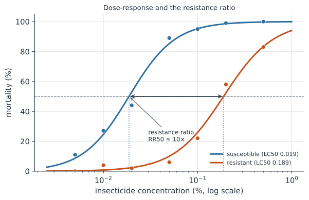
- The intensity or dose-response assay exposes separate batches across a range of concentrations, fits a dose-response curve, and estimates the lethal concentrations and — the doses killing 50% and 90%. Comparing an to that of a susceptible reference strain gives the resistance ratio, a graded measure of intensity (Figure 1).
Diagnostic-dose classification#
The WHO thresholds turn a mortality proportion into a verdict:
| 24-hour mortality | Interpretation |
|---|---|
| susceptible | |
| – | possible resistance (confirm) |
| confirmed resistance |
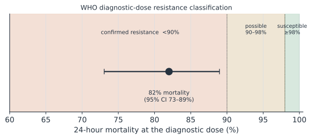
Two statistical points matter. First, mortality is a proportion from a finite sample, so report a binomial confidence interval — with – mosquitoes the interval is wide enough to straddle a threshold. Second, if control (unexposed) mortality is not negligible, correct for it with Abbott’s formula,
discarding the whole test if control mortality exceeds ~20% (Figure 2).
Dose-response and the resistance ratio#
For the dose-response assay, model the number dying out of exposed as binomial with a mortality that rises with log dose — the classic probit (Finney) or the near-identical logit dose-response model:
Inverting it gives the lethal concentrations, e.g. , and the resistance ratio is (with a confidence interval from the two fits).
A worked example#
A diagnostic-dose assay and a full dose-response on a resistant field population versus a susceptible colony.
import numpy as np
from scipy import stats

# --- diagnostic-dose assay: 82 dead of 100, with a small control mortality ---
dead, N, ctrl_dead, ctrl_N = 82, 100, 3, 100
mort = dead / N
ci = stats.binomtest(dead, N).proportion_ci(0.95)
abbott = (mort - ctrl_dead / ctrl_N) / (1 - ctrl_dead / ctrl_N)   # control correction
verdict = ("susceptible" if mort >= 0.98 else
           "possible resistance" if mort >= 0.90 else "confirmed resistance")
print(f"mortality {mort*100:.0f}% (95% CI {ci.low*100:.0f}-{ci.high*100:.0f}%), "
      f"Abbott-corrected {abbott*100:.0f}% -> {verdict}")
mortality 82% (95% CI 73-89%), Abbott-corrected 81% -> confirmed resistance
import statsmodels.api as sm

rng = np.random.default_rng(5)
doses = np.array([0.005, 0.01, 0.02, 0.05, 0.1, 0.2, 0.5])   # % active ingredient
ld = np.log10(doses)

def assay(lc50, slope=4.0, n=100):                            # simulate a strain
    p = 1 / (1 + np.exp(-slope * (ld - np.log10(lc50))))
    return rng.binomial(n, p), np.full(len(doses), n)

def lethal(deaths, n):                                        # fit and invert
    fit = sm.GLM(np.c_[deaths, n - deaths], sm.add_constant(ld),
                 family=sm.families.Binomial()).fit()
    b0, b1 = fit.params
    q = lambda pr: 10 ** ((np.log(pr / (1 - pr)) - b0) / b1)
    return q(0.5), q(0.9)

lc50_s, lc90_s = lethal(*assay(0.02))                         # susceptible colony
lc50_r, lc90_r = lethal(*assay(0.20))                         # resistant field pop
print(f"susceptible LC50={lc50_s:.3f}  resistant LC50={lc50_r:.3f}")
print(f"resistance ratio RR50 = {lc50_r / lc50_s:.1f}")
susceptible LC50=0.019  resistant LC50=0.189
resistance ratio RR50 = 10.1
The population is under-killed at the diagnostic dose (82%, confirmed resistance) and needs roughly ten times the concentration to reach the same — actionable evidence that the deployed insecticide class is losing efficacy.
In code#
R#
# ecotox / drc are the standard dose-response toolkits
library(ecotox)
LC_probit(cbind(dead, alive) ~ log10(dose), p = c(50, 90), data = assay)
# resistance ratio with a CI via drc::ED and the lethal-dose ratio test
library(drc)
m <- drm(dead/total ~ dose, weights = total, fct = LL.2(), type = "binomial")
Julia#
using GLM, DataFrames
m = glm(@formula(dead_frac ~ log10(dose)), df, Binomial(), ProbitLink(), wts = n)
# LC50 = 10^(-coef(m)[1]/coef(m)[2])
Why it matters#
Resistance is now widespread in the major malaria vectors, and a control programme that keeps spraying a compound its mosquitoes no longer die to is wasting money and lives. Diagnostic-dose surveillance flags where resistance has emerged; intensity assays and resistance ratios say how bad it is and whether a higher dose or a different mode of action is needed — the evidence base for insecticide rotations and the WHO’s resistance-management strategy. It is the vector-control counterpart of antimicrobial-resistance monitoring, and it feeds directly into whether the vectorial capacity of a mosquito population can actually be driven down.