The Kalman Filter
The Kalman filter is the exact, closed-form solution to a recurring problem: track a hidden state that drifts over time when all you see is a noisy, indirect measurement of it. It is a two-line recursion — predict where the state is heading, then correct that guess with the new data — that is optimal whenever the dynamics are linear and the noise is Gaussian. For infectious-disease work it is the natural engine for smoothing noisy surveillance signals, estimating a time-varying growth rate or reproduction number, and fusing multiple data streams that arrive at different rates, all with honest uncertainty and near-zero compute.
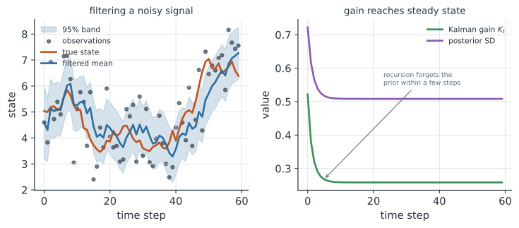
It is also the linear-Gaussian anchor of a whole family of filters. When the model is nonlinear or non-Gaussian — as mechanistic epidemic models usually are — the exact recursion no longer holds, and the particle filter and the POMP inference toolkit take over. The Kalman filter is where that story starts.
The linear-Gaussian state-space model#
The filter assumes a linear-Gaussian state-space model: a hidden state vector that evolves linearly with Gaussian shocks, observed through a linear map with Gaussian noise,
Here is the transition matrix, maps the state to the measurement, and and are the process- and observation-noise covariances. Because everything is linear and Gaussian, the belief about the state stays Gaussian forever, so the filter only ever has to track a mean and covariance — no integrals, no sampling.
The predict–update recursion#
Each step has two halves. First predict: push the previous estimate through the dynamics (1), which moves the mean and inflates the covariance by the process noise,
Then update: fold in the new observation, weighting prediction against data by the Kalman gain ,
The term is the innovation — how much the observation surprised us — and the gain (4) decides how much of that surprise to believe. The gain is a precision-weighted compromise: when the measurement is clean ( small) it pulls the estimate hard toward the data; when the measurement is noisy it barely moves. For a stationary model the gain and covariance settle to a steady state within a handful of steps (the right panel above), so the filter quickly “forgets” its starting guess — which is why the initial prior rarely matters.
A worked example#
Take a scalar local-level model: the state is a slowly wandering quantity (log-incidence, a biomarker level) with process SD (so ), observed with noise SD (so ). Suppose the filter predicts with variance , and the new observation is . The gain is , so the update nudges the estimate only about a quarter of the way to the data: , with variance . Iterating, the gain converges to and the posterior SD to — the filtered signal is half as noisy as the raw observations, which is the smoothing the filter buys you.
In code#
The R version uses the dlm package (with KFAS and MARSS as alternatives), which provides the filter, the smoother, missing-data handling, and the likelihood.
The Python and Julia versions implement the predict–update recursion by hand so the two-line loop is visible.
R#
library(dlm)
set.seed(1)
n <- 60
x_true <- cumsum(rnorm(n, 0, 0.3)) + 5
y <- x_true + rnorm(n, 0, 1)

# local-level model: dV = observation variance, dW = process variance
mod  <- dlmModPoly(order = 1, dV = 1.0, dW = 0.09)
filt <- dlmFilter(y, mod)      # Kalman filter
smoo <- dlmSmooth(filt)        # RTS smoother (uses all the data)

c(filter_rmse = sqrt(mean((dropFirst(filt$m) - x_true)^2)),
  smooth_rmse = sqrt(mean((dropFirst(smoo$s) - x_true)^2)))
Python#
import numpy as np

rng = np.random.default_rng(0)
n = 60
x_true = np.cumsum(rng.normal(0, 0.3, n)) + 5.0     # latent random walk
y = x_true + rng.normal(0, 1.0, n)                  # noisy observations

q, r = 0.09, 1.0                                    # process / obs variance
xhat, P = y[0], 1.0
xf = np.zeros(n)
for t in range(n):
    xp, Pp = xhat, P + q                            # predict
    K = Pp / (Pp + r)                               # Kalman gain
    xhat = xp + K * (y[t] - xp)                     # update
    P = (1 - K) * Pp
    xf[t] = xhat

print(f"steady-state gain     = {K:.3f}")
print(f"filter RMSE vs truth  = {np.sqrt(np.mean((xf - x_true) ** 2)):.3f}")
print(f"raw obs RMSE vs truth = {np.sqrt(np.mean((y - x_true) ** 2)):.3f}")
steady-state gain     = 0.258
filter RMSE vs truth  = 0.626
raw obs RMSE vs truth = 1.013
Julia#
using Random, Statistics

Random.seed!(1)
n = 60
x_true = cumsum(randn(n) .* 0.3) .+ 5
y = x_true .+ randn(n)

q, r = 0.09, 1.0
xhat, P = y[1], 1.0
xf = zeros(n)
for t in 1:n
    xp, Pp = xhat, P + q               # predict
    K = Pp / (Pp + r)                  # Kalman gain
    xhat = xp + K * (y[t] - xp)        # update
    P = (1 - K) * Pp
    xf[t] = xhat
end
sqrt(mean((xf .- x_true).^2))          # filtered RMSE, well below the obs noise
The smoother#
The filter uses only data up to time , which is what you want in real time but wastes information when you are looking back.
The Rauch–Tung–Striebel (RTS) smoother makes a second, backward pass that conditions each state on the entire series, sharpening every estimate and narrowing every band — especially at turning points, where a filter always lags.
Use the filter for nowcasting and forecasting, the smoother for retrospective reconstruction (dlmSmooth above does exactly this).
Going Bayesian: learning the noise#
Everything so far assumed you know the process- and observation-noise variances and — but those are exactly what set the Kalman gain (4), and in practice they are unknown.
Hand-tuning them is the usual fudge; the principled alternative is to put priors on them and let the data decide.
This is where the filter reveals a second gift: as it runs, it produces the exact marginal likelihood of the data given the parameters, , through the innovations (prediction-error) decomposition — it integrates the latent states out analytically, the continuous-Gaussian twin of the HMM forward algorithm.
So we run the Kalman filter inside a NumPyro model to get a smooth log-likelihood in the noise scales and sample their posterior with NUTS — the very objective that dlm and KFAS maximize for MLE, sampled instead of optimized, which also propagates the parameter uncertainty into the state estimates.
Setting priors. The unknowns are two standard deviations, so half-Normal priors — positive and weakly informative — are the natural choice: , with the scale set to the rough magnitude of the data’s fluctuations (an Exponential or half- serves equally well). A prior predictive check confirms those priors imply sensible series before fitting, and a posterior predictive check — here on the standard deviation of the first differences , which for a local-level model equals — confirms the fit reproduces the data’s volatility.
How running the filter marginalizes the latent states — and where that is in the code
A Bayesian sampler needs with the latent states integrated out, and for a linear-Gaussian model that integral is available in closed form — the Kalman filter computes it as a byproduct. As the filter steps forward it produces the one-step-ahead innovation , which is Gaussian with mean zero and variance , and successive innovations are independent. So the marginal likelihood factorizes into a product of these predictive Gaussians — the prediction-error decomposition:
This integrates over all latent-state paths exactly, the Gaussian analogue of the HMM forward algorithm summing over discrete paths — same idea, sum replaced by an integral the Kalman recursion does in closed form.
The kalman_loglik function is precisely this:
- inside
step,xp, Pp = x, P + qis the predict (3);v = yt - xpandS = Pp + rare the innovation and its variance (with for a local level). ll = ll - 0.5*(log(2*pi*S) + v*v/S)accumulates one term of the boxed sum.K = Pp / Sand the returned(xp + K*v, (1-K)*Pp, ll)are the Kalman update (5), carrying the state forward for the next innovation.lax.scanruns the recursion down the series — fast, and differentiable in , which enter only throughqandr— andnumpyro.factor("obs", ...)adds the total to the model’s log-density.
Because the states were integrated out, they are not in the posterior; to recover the filtered/smoothed trajectory you rerun the filter (or the RTS smoother) at the posterior draws, exactly as the HMM recovers its states after marginalizing them.
import numpy as np
import jax.numpy as jnp
from jax import lax, random
import numpyro, numpyro.distributions as dist
from numpyro.infer import MCMC, NUTS

# ---- data: a local-level (random walk + noise) series ----
rng = np.random.default_rng(0)
n = 150
sig_proc_true, sig_obs_true = 0.3, 1.0
x_true = np.cumsum(rng.normal(0, sig_proc_true, n)) + 5.0
y = x_true + rng.normal(0, sig_obs_true, n)
stat = lambda yy: np.std(np.diff(yy))                # SD of first differences
obs_stat = stat(y)


def kalman_loglik(sig_proc, sig_obs, y):
    """Innovations (prediction-error) log-likelihood: marginalizes the states."""
    q, r = sig_proc ** 2, sig_obs ** 2

    def step(carry, yt):
        x, P, ll = carry
        xp, Pp = x, P + q                            # predict
        v, S = yt - xp, Pp + r                       # innovation + its variance
        ll = ll - 0.5 * (jnp.log(2 * jnp.pi * S) + v * v / S)
        K = Pp / S                                   # Kalman gain, then update
        return (xp + K * v, (1 - K) * Pp, ll), None

    (_, _, ll), _ = lax.scan(step, (y[0], 100.0, 0.0), y)
    return ll


def model(y):
    sig_proc = numpyro.sample("sig_proc", dist.HalfNormal(1.0))   # process SD
    sig_obs = numpyro.sample("sig_obs", dist.HalfNormal(1.0))     # observation SD
    numpyro.factor("obs", kalman_loglik(sig_proc, sig_obs, jnp.array(y)))


mcmc = MCMC(NUTS(model), num_warmup=500, num_samples=500, progress_bar=False)
mcmc.run(random.PRNGKey(0), y)
post = mcmc.get_samples()
print("posterior mean [90% CI]:")
for nm, tr in [("sig_proc", sig_proc_true), ("sig_obs", sig_obs_true)]:
    s = np.asarray(post[nm])
    print(f"  {nm:9s} {s.mean():.2f} [{np.percentile(s,5):.2f}, {np.percentile(s,95):.2f}]  truth {tr}")

# ---- prior & posterior predictive checks on the first-difference SD ----
def sim(sp, so, seed):
    r = np.random.default_rng(seed)
    return np.cumsum(r.normal(0, sp, n)) + 5.0 + r.normal(0, so, n)

def pred_interval(sp, so, seed):
    return np.percentile([stat(sim(sp[i], so[i], seed + i)) for i in range(len(sp))], [5, 95])

S = 300; kr = np.random.default_rng(7)
lo0, hi0 = pred_interval(np.abs(kr.normal(0, 1, S)), np.abs(kr.normal(0, 1, S)), 100)  # prior
j = np.random.default_rng(9).integers(0, 500, S)                                        # posterior
lo1, hi1 = pred_interval(np.asarray(post["sig_proc"])[j], np.asarray(post["sig_obs"])[j], 200)
print(f"first-diff SD: observed {obs_stat:.2f}")
print(f"  prior predictive     90% [{lo0:.2f}, {hi0:.2f}]")
print(f"  posterior predictive 90% [{lo1:.2f}, {hi1:.2f}]")
posterior mean [90% CI]:
  sig_proc  0.32 [0.21, 0.48]  truth 0.3
  sig_obs   1.07 [0.97, 1.20]  truth 1.0
first-diff SD: observed 1.54
  prior predictive     90% [0.34, 2.88]
  posterior predictive 90% [1.32, 1.82]
The posterior recovers both noise scales with credible intervals, the prior predictive brackets the observed volatility loosely, and the posterior predictive brackets it tightly — a calibrated fit that learned and from the data instead of by hand. The same recipe extends to the local-linear-trend and multi-stream models above: add priors on their noise scales and run their Kalman filter inside the sampler.
Example: recovering time-varying transmission#
Transmission is never constant — interventions, behavior, and seasonality all move it — so a central task is estimating a time-varying growth rate or reproduction number from a case series. The Kalman filter handles this with a local-linear-trend model: let the log of incidence have both a level and a slope, and make the slope itself a random walk. The slope is exactly the epidemic growth rate , and it maps to the reproduction number through the generation-interval relation (the discrete-time renewal-equation form of the Wallinga–Lipsitch conversion).
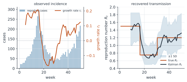
This is a genuinely linear-Gaussian model on the log scale, so the ordinary Kalman filter — no approximations — recovers and its uncertainty.
import numpy as np

rng = np.random.default_rng(8)
T = 50
w = np.array([0.25, 0.35, 0.25, 0.15])          # generation-interval weights
L = len(w)
t = np.arange(T)
R_true = np.where(t < 16, 1.5, np.where(t < 30, 0.75, 1.2))

# renewal-equation incidence, observed at 50% reporting
I = np.zeros(T)
I[:L] = [30, 40, 55, 70]
for k in range(L, T):
    I[k] = rng.poisson(R_true[k] * np.sum(w * I[k - L:k][::-1]))
cases = rng.poisson(0.5 * I)
y = np.log(np.maximum(cases, 1.0))

# local-linear-trend Kalman: state = [level, slope = growth rate r_t]
A = np.array([[1., 1.], [0., 1.]])
H = np.array([1., 0.])
Q = np.diag([1e-3, 8e-3])
Rm = 0.15
x = np.array([y[L], 0.0])
P = np.eye(2) * 0.5
r_hat = np.zeros(T)
for k in range(T):
    x = A @ x
    P = A @ P @ A.T + Q                          # predict
    K = P @ H / (H @ P @ H + Rm)                 # gain
    x = x + K * (y[k] - H @ x)                   # update
    P = (np.eye(2) - np.outer(K, H)) @ P
    r_hat[k] = x[1]

# growth rate -> R_t via the discretized renewal relation
R_est = np.array([1.0 / np.sum(w * np.exp(-r * np.arange(1, L + 1))) for r in r_hat])
print("week  R_true  R_est")
for k in (8, 15, 20, 29, 36, 46):
    print(f"{k + 1:4d}   {R_true[k]:.2f}    {R_est[k]:.2f}")
print(f"RMSE(R_t) = {np.sqrt(np.mean((R_est[L + 2:] - R_true[L + 2:]) ** 2)):.3f}")
week  R_true  R_est
   9   1.50    1.42
  16   1.50    1.54
  21   0.75    0.72
  30   0.75    0.81
  37   1.20    1.22
  47   1.20    1.27
RMSE(R_t) = 0.123
In R the same model is two lines with dlm — a second-order polynomial model whose second state component is the slope:
library(dlm)
# local linear trend on log-cases; component 2 of the state is the growth rate
mod <- dlmModPoly(order = 2, dV = 0.15, dW = c(1e-3, 8e-3))
sm  <- dlmSmooth(log(pmax(cases, 1)), mod)
r_t <- dropFirst(sm$s[, 2])                       # smoothed growth rate
R_t <- 1 / sapply(r_t, function(r) sum(w * exp(-r * seq_along(w))))
The mechanistic route: the ensemble Kalman filter#
The model above is phenomenological — it never mentions , , or . To estimate a time-varying transmission rate inside a mechanistic SIR, you make a random-walk state appended to and filter the augmented system. That dynamic is nonlinear (incidence ), so the plain Kalman filter no longer applies. The extended Kalman filter (EKF) linearizes the dynamics with a Jacobian, but on epidemic models it is notoriously fragile and prone to divergence. The ensemble Kalman filter (EnKF) is the robust workhorse: it represents the state by an ensemble, pushes each member through the exact nonlinear simulator, and computes the Kalman update from the ensemble’s sample covariance — no Jacobian required.
# ensemble Kalman filter over an augmented state (S, I, log beta) — sketch
ens <- init_ensemble(m = 300)                     # draw S, I, log beta
for (t in seq_along(reports)) {
  ens$logbeta <- ens$logbeta + rnorm(300, 0, sigma)   # random walk on log beta
  ens <- sir_step(ens)                                # push through the simulator
  yhat <- rho * ens$new_infections                    # predicted observation
  K    <- cov(cbind(ens$S, ens$I, ens$logbeta), yhat) / (var(yhat) + R_obs)
  ens  <- ens + K %o% (reports[t] + rnorm(300, 0, sqrt(R_obs)) - yhat)  # update
}
This augmented-state EnKF is the method behind operational influenza forecasting (Shaman & Karspeck 2012).
When even a Gaussian ensemble is too crude — strongly nonlinear dynamics, discrete counts, multimodal beliefs — the fully general replacement is the particle filter, and the pomp toolkit fits the same time-varying- model without any Gaussian assumption.
Example: fusing wastewater and case reports#
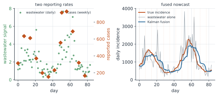
Modern surveillance mixes streams that report at different rates and with different noise: wastewater signal can arrive daily but is very noisy, while confirmed cases arrive weekly and are cleaner but lag. A Kalman filter fuses them effortlessly, because the update step (5) simply runs once per available observation — when a stream is silent, you skip its update, and the filter coasts on the prediction. Both streams are treated as noisy linear reads of one shared latent log-incidence , each with its own scaling constant and variance.
import numpy as np

rng = np.random.default_rng(2)
D = 84
m0 = (np.cumsum(rng.normal(0, 0.06, D)) + np.log(800)
      + 0.7 * np.sin(2 * np.pi * np.arange(D) / 45))
latent = np.exp(m0)                                    # true daily incidence
ww = 0.002 * latent * np.exp(rng.normal(0, 0.45, D))   # daily wastewater (noisy)
cases = np.full(D, np.nan)
for d in range(0, D, 7):                               # cases reported weekly only
    cases[d] = rng.poisson(0.4 * latent[d])

q, r1, r2 = 0.06 ** 2, 0.45 ** 2, 0.12 ** 2            # process / two obs variances
c1, c2 = np.log(0.002), np.log(0.40)                   # stream scaling constants


def run(use_cases):
    m, P = np.log(800), 1.0
    est = np.zeros(D)
    for d in range(D):
        P += q                                         # predict (random walk)
        K = P / (P + r1)                               # update with wastewater (daily)
        m += K * (np.log(ww[d]) - (c1 + m))
        P = (1 - K) * P
        if use_cases and not np.isnan(cases[d]) and cases[d] > 0:
            K = P / (P + r2)                           # update with cases (weekly)
            m += K * (np.log(cases[d]) - (c2 + m))
            P = (1 - K) * P
        est[d] = np.exp(m)
    return est


rmse = lambda e: np.sqrt(np.mean((e - latent) ** 2))
print(f"raw wastewater RMSE  = {rmse(ww / 0.002):6.1f}")
print(f"KF, wastewater only  = {rmse(run(False)):6.1f}")
print(f"KF, fused with cases = {rmse(run(True)):6.1f}")
raw wastewater RMSE  =  540.7
KF, wastewater only  =  373.9
KF, fused with cases =  278.8
The fused estimate is much closer to the truth than either the raw wastewater or the wastewater-only filter — the frequent stream supplies the shape and the sparse stream anchors the level.
In R, dlm (or KFAS) does this natively: stack the two series as columns, mark the missing case-days NA, and the filter skips them automatically.
library(dlm)
z1 <- log(ww) - log(0.002)                 # wastewater, de-scaled to the level
z2 <- log(cases) - log(0.40)               # weekly cases; NA on non-report days
Y  <- cbind(z1, z2)

# one shared random-walk level read by both streams, with their own variances
mod <- dlm(FF = matrix(1, 2, 1), V = diag(c(0.45^2, 0.12^2)),
           GG = 1, W = 0.06^2, m0 = log(800), C0 = 1)
fused <- exp(dropFirst(dlmFilter(Y, mod)$m))   # NA case-days are skipped
Other epidemiological uses#
The same machinery recurs across surveillance and modeling:
- Nowcasting and backfill. Reporting delays mean recent counts are incomplete; a structural time-series Kalman model with a day-of-week component estimates the true recent level and projects the fill-in — see Nowcasting.
- Excess-mortality baselines. A seasonal local-level model gives the expected deaths and a prediction interval; the gap to observed deaths is the excess.
- Within-host viral load. Noisy qPCR / Ct trajectories over time are smoothed into a clean within-host load curve, with the slope estimating growth or clearance rate.
- Multi-signal surveillance. The fusion pattern above extends to any number of streams — ILI, hospitalizations, syndromic, wastewater — each a linear read of a shared latent burden, weighted by its reliability (surveillance systems).
- Data assimilation for forecasting. Cycling an EnKF between mechanistic simulation and observation is the backbone of operational epidemic forecasting.
The wider filtering family#
The Kalman filter is the exact solution at the linear-Gaussian corner; everything else is a way to cope when a model leaves it.
| Filter | Handles | Cost |
|---|---|---|
| Kalman | linear, Gaussian | trivial, exact |
| Extended Kalman (EKF) | mild nonlinearity via Jacobian | cheap, can diverge |
| Unscented Kalman (UKF) | stronger nonlinearity, no Jacobian | cheap, still Gaussian |
| Ensemble Kalman (EnKF) | nonlinear, high-dimensional | moderate, Gaussian update |
| Particle filter | arbitrary nonlinear / non-Gaussian | expensive, general |
The first four keep the Gaussian bookkeeping and differ only in how they push it through nonlinearity; the particle filter drops the Gaussian assumption entirely and samples the belief instead. For mechanistic transmission models — nonlinear, with discrete counts and no closed-form likelihood — that last step is usually necessary, which is where the POMP inference toolkit picks up.
Why it matters#
The Kalman filter is the cheapest honest way to turn a noisy, partial signal into a state estimate with calibrated uncertainty, and an enormous amount of routine epidemiology is exactly that problem: denoising a case series, tracking a growth rate, reconstructing incidence behind reporting delays, combining data streams that disagree. Its predict–update logic — carry a belief forward, then correct it by the data in proportion to their relative precision — is also the conceptual template for every filter that follows, from the ensemble Kalman filters used in flu forecasting to the particle filters behind mechanistic model fitting. Learn it here in its exact, linear-Gaussian form, and the nonlinear generalizations are just the same idea working harder.
Related#
- State-Space Models and Particle Filtering — the nonlinear, non-Gaussian generalization of this page
- POMP Models and Plug-and-Play Inference — fitting mechanistic models when the Kalman assumptions fail
- Hidden Markov Models — the discrete-state analogue, for latent regimes rather than a continuous state
- The Effective Reproduction Number and Forecasting — a prime target of the time-varying-transmission filter
- The Renewal Equation — the growth-rate-to- conversion used above
- Random Walks and Brownian Motion — the process model at the heart of the local-level filter
- Gaussian Processes — the other Gaussian workhorse; a state-space view of GPs yields Kalman-speed inference
- Bayesian Inference · Markov Chain Monte Carlo — the Bayesian fit of the noise variances and its sampler
- Prior Predictive Checks · Posterior Predictive Checks — the checks used on the Bayesian filter
- Nowcasting · Excess Mortality — applications of structural-model filtering
- Quantitative Methods