Life-History Theory and Evolutionary Demography

Life-history theory asks how selection schedules a finite budget of survival and reproduction across an organism’s life: when to mature, how much to reproduce each year, and how long to live. Every allele that raises fecundity now tends to cost survival or future reproduction later, so the schedule that wins is the one that balances these trade-offs, not the one that maximizes any single rate. It is the evolutionary layer that sits on top of demography, and the same logic drives the evolution of virulence, where a pathogen’s “life history” is the balance between transmission and host exploitation.

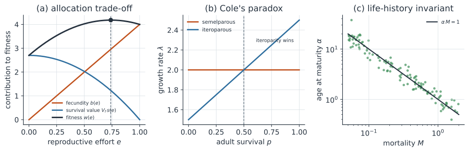
Three panels: a reproductive-effort trade-off with the fitness-maximizing allocation marked; Cole’s paradox comparing the growth rate of semelparous and iteroparous schedules across adult survival; and a life-history-invariant scatter of age at maturity against mortality.

The core trade-off

An organism has a fixed budget of energy and time, and any unit spent on current reproduction cannot also buy growth, maintenance, or survival to the next season. Reproductive effort is the fraction of that budget allocated to current breeding, and the cost of reproduction is the resulting drop in survival and in later fecundity. Selection does not favor maximum effort or maximum caution; it favors the allocation that maximizes lifetime contribution to future generations, weighting a unit of effort now against the future reproduction it forecloses. Stearns (1992, The Evolution of Life Histories, Oxford) frames the whole field as the study of these allocation trade-offs and the constraints that shape them.

Write fitness as the sum of current reproduction and the survival-weighted value of the future,

$w(e) = b(e) + V_f\, s(e),$

where $b(e)$ is fecundity at effort $e$ , $s(e)$ is survival to the next breeding attempt, and $V_f$ is the reproductive value of that future. Because $b$ increases and $s$ decreases with $e$ , the optimum $e^*$ sits where the marginal gain in fecundity just offsets the marginal loss of survival value, $b'(e^*) = -V_f\, s'(e^*)$ .

Cole’s paradox and its resolution

Cole (1954, Quarterly Review of Biology 29:103-137) posed a puzzle: an annual, semelparous genotype that breeds once and dies gains the same increase in growth rate as a perennial, iteroparous genotype that adds just one offspring to each clutch. If a single extra offspring buys the whole advantage of iteroparity, why is any organism perennial at all?

The resolution is that juvenile and adult survival are not equal. Let $c$ be the survival of a newborn to first breeding and $p$ the survival of an adult from one breeding season to the next. A semelparous schedule with clutch $B_s$ has finite growth rate

$\lambda_{\text{semel}} = c\, B_s,$

while an iteroparous schedule with clutch $B_i$ that also survives as an adult has

$\lambda_{\text{itero}} = c\, B_i + p.$

Iteroparity is favored when $\lambda_{\text{itero}} > \lambda_{\text{semel}}$ , i.e.

$p > c\,(B_s - B_i).$

Cole assumed $c = 1$ , which collapses the condition to needing $B_s = B_i + 1$ and makes semelparity look nearly free. Once juveniles survive worse than adults, holding onto a reliable adult (large $p$ ) beats gambling on a batch of cheap juveniles, and iteroparity is favored whenever adult survival is high relative to juvenile survival.

Optimization by reproductive value

The right currency for these comparisons is a fitness measure that selection actually maximizes, usually the intrinsic rate of increase $r$ or the lifetime reproduction $R_0$ . For an age-structured schedule with survivorship $l(a)$ and age-specific fecundity $m(a)$ , $r$ solves the Euler-Lotka equation,

$\sum_{a} e^{-r a}\, l(a)\, m(a) = 1.$

Delaying maturity to age $\alpha$ has two effects that pull against each other: it postpones and shortens the reproductive span, discounting future offspring by $e^{-r a}$ and by the survivorship $l(\alpha)$ needed to reach $\alpha$ , but it can raise fecundity if the organism keeps growing. The optimal $\alpha$ balances the marginal fecundity gained by waiting against the marginal survival and discounting lost, each weighted by reproductive value, so a change is favored only when it raises $r$ summed over the whole schedule.

r/K selection and life-history invariants

Species array along a fast-slow continuum: fast (r-selected) life histories mature early, breed hard, and die young; slow (K-selected) life histories mature late, breed cautiously, and live long. Charnov (1993, Life History Invariants, Oxford) showed that when the underlying trade-offs scale the same way across taxa, certain dimensionless combinations stay nearly constant. The clearest example is the product of age at maturity $\alpha$ and adult mortality $M$ ,

$\alpha\, M \approx \text{constant},$

so a mouse and an elephant, despite a thousand-fold difference in lifespan, mature at roughly the same fraction of their expected adult life. Such invariants are the signature of an optimized trade-off: rescale mortality and the optimal schedule rescales with it, leaving the dimensionless ratio fixed.

A worked example

Take Cole’s comparison with juvenile survival $c = 0.4$ and a semelparous clutch one offspring larger than the iteroparous one, $B_s - B_i = 1$ . The condition $p > c\,(B_s - B_i) = 0.4$ says iteroparity wins as soon as adult survival exceeds $0.4$ , even though the semelparous genotype produces more offspring per attempt.

For the age at maturity, take survivorship $l(a) = e^{-Ma}$ with $M = 0.3$ and fecundity that grows with body size as $m(\alpha) = 0.1\,\alpha^2$ once breeding starts. Sweeping $\alpha$ and solving Euler-Lotka for $r$ at each value gives an interior optimum at $\alpha^* = 5$ with $r^* \approx 0.104$ : maturing at one gives a negative growth rate because the animal is tiny and barely fecund, while maturing at twelve wastes too many years to mortality, and the balance lands in between.

In code

We sweep the age at maturity, solve the Euler-Lotka equation for $r$ at each value, and locate the optimum.

R

M <- 0.3; B0 <- 0.1; ages <- 1:40

growth_rate <- function(alpha) {
  b <- B0 * alpha^2            # fecundity grows with body size
  a <- ages[ages >= alpha]
  l <- exp(-M * a)             # survivorship under mortality M
  uniroot(function(r) sum(exp(-r * a) * l * b) - 1,
          c(-1, 5))$root
$}

grid <- 1:12
r <- sapply(grid, growth_rate)
grid[which.max(r)]            # 5 = optimal age at maturity
max(r)                        # ~0.104

Python

import numpy as np
from scipy.optimize import brentq
import polars as pl

M, B0, T = 0.3, 0.1, 40           # mortality, fecundity scale, max age
ages = np.arange(1, T + 1)

def growth_rate(alpha):
    # Euler-Lotka: sum_a exp(-r a) l(a) b(alpha) = 1, reproduce from alpha on.
    b = B0 * alpha**2             # growth: body size (hence fecundity) rises
    a = ages[ages >= alpha]
    l = np.exp(-M * a)            # survivorship under constant mortality M
    f = lambda r: np.sum(np.exp(-r * a) * l * b) - 1.0
    return brentq(f, -1.0, 5.0)

grid = np.arange(1, 13)
r = np.array([growth_rate(al) for al in grid])
best = grid[np.argmax(r)]
tab = pl.DataFrame({"alpha": grid, "r": np.round(r, 4)})
print(tab.filter(pl.col("alpha").is_in([1, 3, best, best + 3, 12])))
print("optimal age at maturity:", best, " r* =", round(r.max(), 4))

shape: (5, 2)
┌───────┬─────────┐
│ alpha ┆ r       │
│ ---   ┆ ---     │
│ i64   ┆ f64     │
╞═══════╪═════════╡
│ 1     ┆ -0.2069 │
│ 3     ┆ 0.0621  │
│ 5     ┆ 0.1037  │
│ 8     ┆ 0.0768  │
│ 12    ┆ 0.0284  │
└───────┴─────────┘
optimal age at maturity: 5  r* = 0.1037

Julia

using Roots

M, B0, ages = 0.3, 0.1, 1:40

function growth_rate(alpha)
    b = B0 * alpha^2                 # fecundity grows with body size
    a = ages[ages .>= alpha]
    l = exp.(-M .* a)                # survivorship under mortality M
    find_zero(r -> sum(exp.(-r .* a) .* l .* b) - 1, (-1.0, 5.0))
end

grid = 1:12
r = growth_rate.(grid)
grid[argmax(r)]                      # 5 = optimal age at maturity
maximum(r)                           # ~0.104

Why it matters

Life-history theory explains why organisms are neither immortal breeders nor one-shot maximizers: a fixed budget forces trade-offs, and selection tunes the schedule of survival and reproduction to the mortality regime an organism faces. The same accounting drives pathogen evolution, where transmission plays the role of fecundity and host survival the role of parental survival, so the evolution of virulence is a life-history problem solved in the currency of $R_0$ . Reading demographic rates through the lens of reproductive value and the Euler-Lotka equation turns a species’ survival and fecundity schedule into a prediction about how it will evolve, and turns interventions that change those rates into predictions about how the organism will respond.