Matching Methods

Matching removes confounding at the design stage: before looking at outcomes, you build a comparison group whose covariates look like the treated group’s, so the treated-versus-control contrast is no longer distorted by the things that drove treatment. It is the most transparent of the propensity-era tools — you can literally inspect who was matched to whom — and it complements weighting and g-estimation as a way to answer the same causal question. This page covers the three matching flavors you will actually meet.

Figure 1. Standardized mean differences for three confounders: large before matching (treated and control groups differ), and collapsed toward zero after both propensity-score matching and coarsened exact matching. The dashed lines at ±0.1 are the usual balance rule-of-thumb.

Exact matching#

The purest form pairs each treated unit with controls having identical covariate values. It is unbeatable when it works — no modelling, perfect balance — but it collapses under the curse of dimensionality: with several covariates, or any continuous one, almost no two units match exactly, and most of the sample is discarded. The other two methods are both ways of relaxing “identical” into “similar enough.”

Propensity-score matching#

Instead of matching on the whole covariate vector, match on the scalar propensity score $\hat e(L)$ — the balancing score, so units with the same propensity have the same covariate distribution. The common recipe is nearest-neighbor matching: for each treated unit, take the control with the closest propensity (often on the logit scale), optionally within a caliper (a maximum allowed distance) to refuse bad matches. Variants trade bias against variance — $1{:}k$ matching, matching with or without replacement, and optimal/full matching that minimizes total distance rather than greedily. Matching each treated unit to a control estimates the effect on the treated (ATT), the usual target of a matched analysis.

Coarsened exact matching#

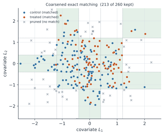
Coarsened exact matching (CEM, Iacus, King & Porro 2012) takes the opposite route: coarsen each covariate into substantive bins (age decades, income brackets), exact-match on the coarsened values, and keep only the strata containing both treated and control units — pruning the rest (Figure 2).

Figure 2. Coarsening carves the covariate space into cells; treated and control units are exact-matched within cells. Cells holding both groups are kept (shaded); units in cells with only one group are pruned. This bounds imbalance directly, with no propensity model.

CEM has two attractive properties:

Monotonic imbalance bounding: you choose the coarseness, which directly caps the imbalance on each covariate — tighter bins mean better balance and more pruning, a knob you control rather than discover after fitting a model.
No propensity model: nothing to mis-specify; balance is a property of the coarsening, not of a fitted regression.

The cost is the pruning: dropping unmatched units shifts the estimand toward the region of common support and shrinks the sample, so report how many units survived.

Checking balance, not significance#

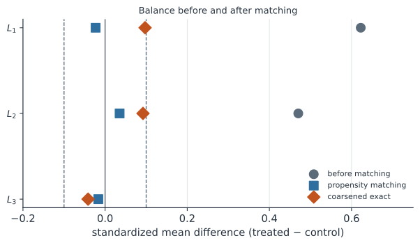
Whatever the method, the deliverable is balance, summarized by the standardized mean difference (SMD) — the difference in covariate means between groups, in pooled-SD units — before and after matching, displayed as a “love plot” (Figure 1). A conventional target is $|\text{SMD}| < 0.1$ . Do not use hypothesis tests of balance: they conflate balance with sample size, and matching changes both.

A worked example#

On confounded data with three covariates, both propensity matching and CEM restore balance and recover the true effect ( $-2$ ).

Python

import numpy as np
import statsmodels.api as sm
from collections import defaultdict

rng = np.random.default_rng(4)
n = 2000
L1, L2, L3 = rng.normal(0, 1, n), rng.normal(0, 1, n), rng.normal(0, 1, n)
A = rng.binomial(1, 1 / (1 + np.exp(-(0.7 * L1 + 0.6 * L2 - 0.4 * L3))))
Y = -2.0 * A + 1.0 * L1 + 0.8 * L2 + 0.5 * L3 + rng.normal(0, 1, n)   # true ATT = -2
X = np.column_stack([L1, L2, L3])
tr, co = np.where(A == 1)[0], np.where(A == 0)[0]

def smd(xt, xc, wc=None):
    return np.array([(xt[:, j].mean()
                      - (xc[:, j].mean() if wc is None else np.average(xc[:, j], weights=wc)))
                     / np.sqrt((xt[:, j].var() + xc[:, j].var()) / 2) for j in range(3)])

# propensity-score nearest-neighbour matching (logit scale)
lps = np.log((e := sm.Logit(A, sm.add_constant(X)).fit(disp=0).predict()) / (1 - e))
mc = np.array([co[np.argmin(np.abs(lps[co] - lps[i]))] for i in tr])
print(f"before  |SMD| max {np.abs(smd(X[tr], X[co])).max():.2f}")
print(f"PS match |SMD| max {np.abs(smd(X[tr], X[mc])).max():.2f}   ATT {np.mean(Y[tr]-Y[mc]):+.2f}")

# coarsened exact matching on covariate quartiles
bins = [np.quantile(X[:, j], [.25, .5, .75]) for j in range(3)]
strata = defaultdict(lambda: ([], []))
for i in range(n):
    strata[tuple(int(np.digitize(X[i, j], bins[j])) for j in range(3))][A[i]].append(i)
num = den = 0; kt = []; kc = []; wc = []
for cc, ct in strata.values():
    if cc and ct:
        num += (Y[ct].mean() - Y[cc].mean()) * len(ct); den += len(ct)
        kt += ct; kc += cc; wc += [len(ct) / len(cc)] * len(cc)
print(f"CEM     |SMD| max {np.abs(smd(X[np.array(kt)], X[np.array(kc)], np.array(wc))).max():.2f}"
      f"   ATT {num/den:+.2f}   kept {len(kt)}/{len(tr)}")

before  |SMD| max 0.62
PS match |SMD| max 0.04   ATT -1.95
CEM     |SMD| max 0.10   ATT -1.83   kept 991/991

Both drive the worst covariate imbalance well below $0.1$ and recover an ATT near $-2$ ; propensity matching balances a touch tighter here, while CEM guarantees its balance by construction and needs no propensity model.

In code#

R#

library(MatchIt)
# nearest-neighbour propensity matching with a caliper
m_ps  <- matchit(A ~ L1 + L2 + L3, data = d, method = "nearest",
                 distance = "glm", caliper = 0.2)
# coarsened exact matching (method = "cem")
m_cem <- matchit(A ~ L1 + L2 + L3, data = d, method = "cem")
summary(m_ps)                         # standardized mean differences before/after
library(cobalt); love.plot(m_cem)     # the balance love plot

Julia#

Julia

# match on the estimated propensity (logit scale), nearest neighbour
using GLM, DataFrames
e = predict(glm(@formula(A ~ L1 + L2 + L3), d, Binomial()))
lps = log.(e ./ (1 .- e))
# for each treated unit pick the control minimizing |lps_t - lps_c|

Why it matters#

Matching is the causal method that most resembles the trial it is imitating: it constructs, from observational data, two groups that differ (as far as the measured covariates go) only in treatment, and it lets you see and defend that comparison before any outcome is analyzed. Propensity matching and CEM are the two that scale — the first by collapsing covariates to a score, the second by coarsening them to bins — and they fail in the same honest way, by refusing to match units with no counterpart rather than extrapolating. As with every method on these pages, matching balances only what you measured; the units it cannot match are a feature, flagging where the data simply cannot answer the question.