Meta-Regression

A meta-analysis that finds high heterogeneity has raised a question, not answered one: why do the studies disagree? Meta-regression is the tool for answering it — a random-effects regression of the study effect sizes on study-level covariates (moderators), asking whether differences in dose, setting, year, latitude, or population explain the scatter. It is the meta-analytic counterpart of adding predictors to a regression, with one twist: each “observation” is a whole study, weighted by its precision.

The model#

Extend the random-effects model so each study’s true effect depends on its moderator $x_i$ :

$y_i = \beta_0 + \beta_1 x_i + u_i + \varepsilon_i, \qquad u_i \sim \mathcal{N}(0, \tau^2_{\text{resid}}),\ \varepsilon_i \sim \mathcal{N}(0, v_i),$

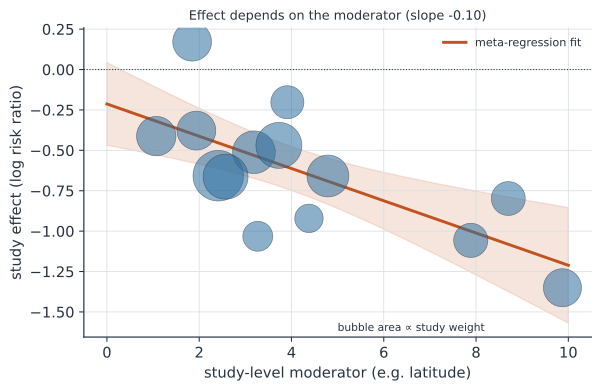
where $v_i$ is the within-study variance and $\tau^2_{\text{resid}}$ is the residual between-study variance left after accounting for the moderator. Each study is weighted by $w_i = 1/(v_i + \tau^2_{\text{resid}})$ — inverse of its total variance — so precise studies count more, exactly as in ordinary meta-analysis, and the slope $\beta_1$ is estimated by weighted least squares (Figure 1).

How much heterogeneity is explained#

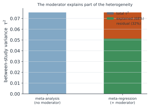
The payoff is comparing the between-study variance before and after adding the moderator. Fit the intercept-only model to get the total heterogeneity $\tau^2_{\text{total}}$ , then the meta-regression to get the residual $\tau^2_{\text{resid}}$ ; the fraction explained is a meta-analytic $R^2$ ,

$R^2 = 1 - \frac{\tau^2_{\text{resid}}}{\tau^2_{\text{total}}},$

the share of the true-effect variance the moderator accounts for (Figure 2). A residual $\tau^2 > 0$ means the studies still differ for reasons your moderator does not capture — the usual outcome, since one covariate rarely explains everything.

Figure 2. The total between-study variance splits into a part explained by the moderator and a residual part. Here the moderator accounts for about two-thirds of the heterogeneity, but a third remains unexplained.

Two traps#

Warning

Ecological fallacy (aggregation bias). A meta-regression relates study-average moderators to study-average effects; the association across studies need not hold within them. A drug that works better in trials with older average age does not necessarily work better in older individuals — only individual-participant-data meta-analysis can settle that.

Warning

Too few studies. Heterogeneity is hard to estimate and moderators are easy to fit spuriously. A common rule of thumb is at least ~10 studies per covariate; with fewer, a “significant” moderator is often noise, and testing many moderators invites false positives.

A worked example#

Fourteen studies report a log risk ratio, with a study-level moderator (say latitude) that genuinely shifts the effect.

Python

import numpy as np

rng = np.random.default_rng(8)
k = 14
x = rng.uniform(0, 10, k)                       # study-level moderator
se = rng.uniform(0.12, 0.35, k)
y = -0.15 - 0.10 * x + rng.normal(0, 0.05, k) + rng.normal(0, se)   # effects
v = se**2

def re_meta(X):                                 # DerSimonian-Laird meta-regression
    w = 1 / v
    b = np.linalg.lstsq(X * np.sqrt(w)[:, None], y * np.sqrt(w), rcond=None)[0]
    Q = np.sum(w * (y - X @ b) ** 2)
    H = np.linalg.inv(X.T @ (w[:, None] * X))
    tr = np.sum(w) - np.trace(H @ (X.T @ ((w**2)[:, None] * X)))
    tau2 = max(0.0, (Q - (k - X.shape[1])) / tr)
    ws = 1 / (v + tau2)                          # refit with random-effects weights
    b = np.linalg.lstsq(X * np.sqrt(ws)[:, None], y * np.sqrt(ws), rcond=None)[0]
    se_b = np.sqrt(np.diag(np.linalg.inv(X.T @ (ws[:, None] * X))))
    return b, se_b, tau2

_, _, tau2_total = re_meta(np.ones((k, 1)))                      # no moderator
b, se_b, tau2_resid = re_meta(np.column_stack([np.ones(k), x]))  # with moderator
print(f"slope {b[1]:.3f} (SE {se_b[1]:.3f})")
print(f"total tau^2 {tau2_total:.3f}  residual tau^2 {tau2_resid:.3f}  "
      f"R2 {(1 - tau2_resid / tau2_total) * 100:.0f}%")

slope -0.100 (SE 0.028)
total tau^2 0.076  residual tau^2 0.024  R2 68%

The moderator has a clear negative slope and explains most — but not all — of the heterogeneity; the residual $\tau^2$ that remains is the honest signal that other, unmeasured differences between studies are still at work.

In code#

R#

library(metafor)
m0 <- rma(yi, vi, data = d)                 # random-effects meta-analysis
m1 <- rma(yi, vi, mods = ~ latitude, data = d)   # meta-regression
m1                                          # slope, residual tau^2, R^2
regplot(m1)                                 # the bubble plot

Julia#

Julia

using GLM, DataFrames
# weighted least squares with weights 1/(v + tau^2); estimate tau^2 by DerSimonian-Laird
wls = lm(@formula(y ~ x), d, wts = 1 ./ (d.v .+ tau2))

Why it matters#

Pooling studies into a single number is often the least interesting thing a meta-analysis can do; the scientific payoff is usually in the heterogeneity — for whom, where, and under what conditions does the effect change? Meta-regression is how evidence synthesis moves from “what is the average effect” to “what explains the differences,” informing which populations a vaccine or drug helps most and where more trials are needed. Handled carelessly — too few studies, or read as individual-level causation — it manufactures spurious moderators; handled well, it turns a discouraging $I^2$ into a finding.