Propensity Scores

In a randomized trial, treatment is assigned by a coin, so treated and control groups are comparable and a simple difference in outcomes estimates the causal effect. In an observational study treatment is chosen — sicker patients get the drug, richer districts get the programme — so the groups differ in ways that also affect the outcome, and a naive comparison is confounded. The propensity score is the single most useful device for fixing this when the confounders are measured.

Figure 1. Every principled propensity method recovers the true effect while the naive comparison does not: against a true effect of −2, a crude treated-minus-control difference is confounded (about −0.9), but propensity matching, stratification, and weighting all land near −2.

The balancing score#

The propensity score is the probability of receiving treatment given the measured confounders $L$ :

$e(L) = \Pr(A = 1 \mid L).$

Its magic property (Rosenbaum & Rubin 1983) is that it is a balancing score: among units with the same propensity, the distribution of $L$ is the same in the treated and control groups. So conditioning on the single scalar $e(L)$ balances the entire vector of confounders — you have reduced a high-dimensional adjustment problem to one dimension. In practice $e(L)$ is unknown and estimated, usually by logistic regression of $A$ on $L$ (or a flexible learner).

Two assumptions make this causal, and neither is testable from the data:

No unmeasured confounding (ignorability): $L$ contains all common causes of $A$ and $Y$ .
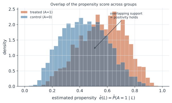
Positivity / overlap: $0 < e(L) < 1$ for all $L$ — every unit could have received either treatment, so the groups’ propensity distributions overlap (Figure 2).

Figure 2. The estimated propensity plotted separately for treated and control units: the distributions differ (that is the confounding) but overlap across the whole range, so every treated unit has comparable controls. That overlap is the positivity assumption.

Four ways to use it#

Once you have $\hat e(L)$ , there are four standard ways to remove confounding with it:

Matching — pair each treated unit with a control of (nearly) the same propensity, then compare within pairs.
Stratification — split the sample into propensity strata (often quintiles) and average the within-stratum treatment–control differences.
Weighting — reweight units by the inverse of their propensity to build a balanced pseudo-population; this is inverse probability weighting, its own page.
Covariate adjustment — include $\hat e(L)$ as a regressor.

Tip

Combining a propensity model with an outcome model gives a doubly robust estimator (augmented IPW): it is consistent if either the propensity model or the outcome model is correct, not necessarily both — a valuable insurance policy.

A worked example#

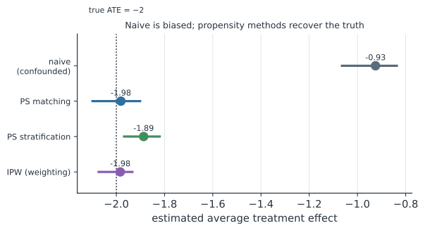
A treatment that truly lowers the outcome by $2$ is preferentially given to units with higher $L$ , and $L$ also raises the outcome — so the naive comparison is badly biased toward zero. Estimating the propensity and applying matching and stratification recovers the true effect.

Python

import numpy as np
import statsmodels.api as sm

rng = np.random.default_rng(2)
n = 4000
L = rng.normal(0, 1, n)                          # measured confounder
A = rng.binomial(1, 1 / (1 + np.exp(-0.8 * L)))  # treatment depends on L
Y = -2.0 * A + 1.5 * L + rng.normal(0, 1, n)     # true ATE = -2; L also affects Y

ehat = sm.Logit(A, sm.add_constant(L)).fit(disp=0).predict()   # propensity model

naive = Y[A == 1].mean() - Y[A == 0].mean()

# stratification on propensity quintiles
q = np.quantile(ehat, np.linspace(0, 1, 6)); q[0] -= 1e-9
strata = np.digitize(ehat, q[1:-1])
diffs, sizes = [], []
for s in np.unique(strata):
    m = strata == s
    diffs.append(Y[m][A[m] == 1].mean() - Y[m][A[m] == 0].mean()); sizes.append(m.sum())
strat = np.average(diffs, weights=sizes)

# nearest-neighbour matching on the propensity
co = np.where(A == 0)[0]; ec = ehat[co]
match = np.mean([Y[i] - Y[co[np.argmin(np.abs(ec - ehat[i]))]]
                 for i in np.where(A == 1)[0]])

print(f"naive (confounded) {naive:+.2f}")
print(f"PS stratification  {strat:+.2f}")
print(f"PS matching        {match:+.2f}   (true -2.00)")

naive (confounded) -0.93
PS stratification  -1.89
PS matching        -1.98   (true -2.00)

The naive estimate is confounded almost to nothing; both propensity methods recover the true $-2$ . The whole approach lives or dies on the balance it achieves — always check that covariates are actually balanced after matching or weighting (a standardized-difference “love plot”), not just that a model was fit.

In code#

R#

library(MatchIt)      # matching, weighting, and balance diagnostics in one place
m <- matchit(A ~ L, data = d, method = "nearest", distance = "glm")
summary(m)            # standardized mean differences before/after (check balance)
# WeightIt + cobalt for weighting and love plots; twang for boosted propensity models

Julia#

Julia

using GLM, DataFrames
ps = predict(glm(@formula(A ~ L), d, Binomial()))   # propensity score
# stratify on quantiles of ps, or pass ps to a matching/weighting routine

Why it matters#

Most epidemiological questions cannot be randomized — you cannot assign people to smoke, to live near a factory, or to miss a vaccine — so causal inference leans heavily on adjusting for measured confounders, and the propensity score is the workhorse for doing it transparently. Its great virtue is separating design from analysis: you build and check the propensity model, confirming balance, before ever looking at the outcome, which disciplines the analysis the way randomization disciplines a trial. Its great limitation is the untestable no-unmeasured-confounding assumption — propensity methods make the measured confounders comparable, and can do nothing about the ones you did not measure.

Propensity Scores

The balancing score#

Four ways to use it#

A worked example#

In code#

R#

Julia#

Why it matters#

Related#