Convolutional Networks and Image Identification

A photograph of a skin lesion is tens of thousands of pixels, and a plain multilayer perceptron that treated each pixel as an independent input would need a colossal number of weights and would still be blind to the fact that a feature means the same thing wherever it appears. A convolutional neural network (CNN) exploits the structure of images directly: it slides small learned filters across the image, detecting the same local pattern — an edge, a texture, a colour transition — everywhere at once. Stack these layers and the network builds understanding hierarchically, from edges to shapes to lesion-level features, which is what lets CNNs read radiographs, count cells, and flag a suspicious mole.

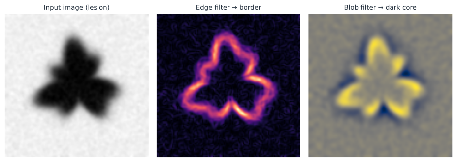
The convolution operation#

The core operation slides a small filter (or kernel) $\mathbf{K}$, say $3\times 3$, across the image $\mathbf{I}$ and, at each position, computes a weighted sum of the pixels under it: $$(\mathbf{I} * \mathbf{K})_{ij} = \sum_{m}\sum_{n} \mathbf{I}_{i+m,\,j+n}\, \mathbf{K}_{m,n}. \tag{1}$$ The output is a feature map that is large where the local image patch resembles the filter. Three properties make this the right operation for images. The filter is local, looking at a small neighbourhood, matching how visual features are local. Its weights are shared across all positions, so the same edge detector applies everywhere — far fewer parameters than a dense layer, and built-in translation equivariance (a feature shifted in the image shifts in the feature map). And the filters are learned by backpropagation, not hand-designed: the network discovers which patterns are worth detecting for the task.

A convolutional layer applies many filters, producing a stack of feature maps, and passes them through a nonlinear activation (usually ReLU).

Pooling and depth#

Between convolutions a pooling step downsamples each feature map — max pooling keeps the strongest response in each small window — shrinking the spatial resolution while retaining what was detected. Pooling buys a measure of translation invariance and lets deeper layers see a larger effective region of the original image. A typical CNN alternates convolution and pooling several times, so that early layers respond to edges and colour, middle layers to textures and motifs (the ragged border, the asymmetry), and late layers to whole-object concepts. A final few dense layers map the top feature maps to class probabilities — “melanoma” versus “benign nevus”, say — through a softmax.

Transfer learning#

Training a deep CNN from scratch needs enormous labelled datasets, which clinical imaging rarely has. Transfer learning solves this: take a network already trained on millions of general images (its early layers have learned reusable edge and texture detectors), replace its final classification layer, and fine-tune on your smaller medical dataset. The generic visual features transfer, so a dermatology classifier can be trained on thousands rather than millions of images — the standard recipe for medical-imaging models today.

A worked example#

Apply a vertical-edge filter $\mathbf{K} = \begin{bmatrix} 1 & 0 & -1 \\ 2 & 0 & -2 \\ 1 & 0 & -1 \end{bmatrix}$ to a $3\times 3$ patch that straddles a light–dark boundary, $\mathbf{I} = \begin{bmatrix} 9 & 9 & 1 \\ 9 & 9 & 1 \\ 9 & 9 & 1 \end{bmatrix}$. By (1) the response is $1\cdot 9 + 0\cdot 9 + (-1)\cdot 1 + 2\cdot 9 + 0\cdot 9 + (-2)\cdot 1 + 1\cdot 9 + 0\cdot 9 + (-1)\cdot 1 = 9-1+18-2+9-1 = 32$, a large positive value flagging the vertical edge. A uniform patch (all $9$s) would give $1\cdot9 - 1\cdot9 + 2\cdot9 - 2\cdot9 + 1\cdot9 - 1\cdot9 = 0$: the filter fires on the transition, not the flat region. Stacking millions of such responses, learned rather than fixed, is all a CNN is doing.

In code#

Python#

Convolution itself is a few lines — here the vertical-edge filter from the worked example run over a small image, showing the feature map that lights up the boundary:

import numpy as np
from scipy.signal import correlate2d

img = np.array([[9, 9, 9, 1, 1],
                [9, 9, 9, 1, 1],
                [9, 9, 9, 1, 1],
                [9, 9, 9, 1, 1],
                [9, 9, 9, 1, 1]], dtype=float)
kernel = np.array([[1, 0, -1], [2, 0, -2], [1, 0, -1]])   # vertical-edge detector
feature_map = correlate2d(img, kernel, mode="valid")       # CNNs cross-correlate
print("feature map (edge responses):")
print(feature_map.astype(int))

feature map (edge responses):
[[ 0 32 32]
 [ 0 32 32]
 [ 0 32 32]]

For a runnable image-classification demonstration we use scikit-learn on the 8×8 handwritten-digit images — a small stand-in for a real diagnostic image set — training a network to identify each image’s class:

from sklearn.datasets import load_digits
from sklearn.model_selection import train_test_split
from sklearn.neural_network import MLPClassifier

digits = load_digits()                                  # 1797 8x8 grayscale images
Xtr, Xte, ytr, yte = train_test_split(digits.data, digits.target,
                                      test_size=0.3, random_state=0)
clf = MLPClassifier(hidden_layer_sizes=(64,), max_iter=800,
                    random_state=0).fit(Xtr, ytr)
print(f"image classification test accuracy: {clf.score(Xte, yte):.3f}")

image classification test accuracy: 0.969

An actual convolutional network — convolution, pooling, then a dense head — trains in PyTorch on those same 8×8 digit images (reshaped to one-channel pictures), showing the real architecture at work:

import torch, torch.nn as nn
torch.manual_seed(0)

def as_images(a):                                    # (N, 64) -> (N, 1, 8, 8), scaled
    return torch.tensor(a.reshape(-1, 1, 8, 8) / 16.0, dtype=torch.float32)
Xtr_t, Xte_t = as_images(Xtr), as_images(Xte)
ytr_t = torch.tensor(ytr, dtype=torch.long)

cnn = nn.Sequential(
    nn.Conv2d(1, 8, 3, padding=1), nn.ReLU(), nn.MaxPool2d(2),    # 8x8 -> 4x4
    nn.Conv2d(8, 16, 3, padding=1), nn.ReLU(), nn.MaxPool2d(2),   # 4x4 -> 2x2
    nn.Flatten(), nn.Linear(16 * 2 * 2, 10))
opt = torch.optim.Adam(cnn.parameters(), lr=0.01)
for epoch in range(150):
    opt.zero_grad()
    loss = nn.functional.cross_entropy(cnn(Xtr_t), ytr_t)
    loss.backward(); opt.step()
acc = (cnn(Xte_t).argmax(1).numpy() == yte).mean()
print(f"CNN test accuracy: {acc:.2f}  (> 0.95: {bool(acc > 0.95)})")

CNN test accuracy: 0.98  (> 0.95: True)

A real dermatology classifier does not train from scratch — it fine-tunes a pretrained backbone via transfer learning; the idiomatic pipeline in PyTorch/torchvision (illustrative — it fetches ImageNet weights over the network, so it is shown, not run here):

# no-run
import torch, torch.nn as nn
from torchvision import models

net = models.efficientnet_b0(weights="IMAGENET1K_V1")    # transferred features
for p in net.parameters():
    p.requires_grad = False                              # freeze the backbone
net.classifier[1] = nn.Linear(net.classifier[1].in_features, 2)  # benign vs malignant
opt = torch.optim.Adam(net.classifier.parameters(), lr=1e-3)
# ... fine-tune net on HAM10000 / ISIC images, tracking validation AUC ...

R#

# keras3 mirrors the Python API; transfer learning from a pretrained backbone.
library(keras3)
base <- application_efficientnet_b0(include_top = FALSE, weights = "imagenet",
                                    input_shape = c(224, 224, 3))
freeze_weights(base)
model <- keras_model_sequential() |>
  base() |>
  layer_global_average_pooling_2d() |>
  layer_dense(units = 2, activation = "softmax")

Julia#

# Flux + Metalhead provides pretrained CNN backbones for transfer learning.
using Flux, Metalhead
backbone = ResNet(18; pretrain = true).layers[1]
model = Chain(backbone, AdaptiveMeanPool((1, 1)), Flux.flatten,
              Dense(512 => 2), softmax)

Why it matters, and where it misleads#

CNNs are transforming diagnostic imaging: dermatology (classifying skin lesions from photographs, using datasets such as HAM10000 and the ISIC archive), radiology (tuberculosis on chest X-rays, fractures, haemorrhages), pathology (tumour detection on whole-slide images), and ophthalmology (diabetic retinopathy from fundus photos), several now at or above specialist accuracy on curated test sets. For infectious disease this reaches into the field: automated reading of malaria blood smears, identifying mosquito species or vector habitat from images, and phone-based triage of rashes where dermatologists are scarce.

But a medical image classifier is exactly where machine learning’s failure modes bite hardest, so the caveats are not optional. Dermatology training sets have historically under-represented darker skin tones, and a model that never saw them will fail on the patients who can least afford a missed melanoma. CNNs latch onto spurious correlates — a model has learned to call lesions malignant because clinicians placed a ruler beside worrying ones, keying on the ruler, not the lesion. Performance on a curated benchmark rarely survives the shift to a new clinic’s camera, lighting, and patient mix, so external, prospective validation is essential before any clinical claim. And a confident probability is not a calibrated one: these tools belong as a second reader that flags and defers to a clinician, not as an autonomous diagnosis. The mathematics is powerful; the responsibility is in how honestly it is validated and deployed.

Related#

• Neural Networks and the Multilayer Perceptron
• Deep Learning, Foundation Models, and Agentic AI
• Diagnostic Testing and Screening
• Proper Scoring Rules
• Variational Autoencoders
• Recurrent Networks and LSTMs
• Quantitative Methods