Sampling Distributions

A statistic computed from a sample is itself random: draw a new sample and you get a new value. The distribution of that statistic over repeated samples — its sampling distribution — is the bridge from a single estimate to a statement about uncertainty.

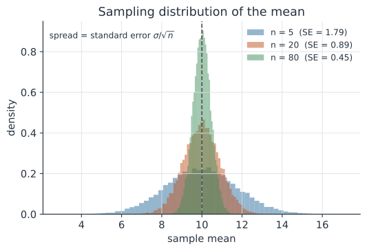
The sampling distribution of the mean narrows as the sample size increases (standard error ). — Figure 1. The sampling distribution of the mean narrows as the sample size $n$ increases (standard error $\sigma/\sqrt{n}$ ).

The idea#

Fix a population and a sample size $n$ . Any statistic, say the sample mean $\bar{X}$ , changes from sample to sample. If you could repeatedly draw fresh samples of size $n$ and recompute $\bar{X}$ each time, the histogram of those values is the sampling distribution of $\bar{X}$ .

It is a distribution of an estimator, not of raw data. Its spread measures how precise the estimate is.

Sampling distribution of the mean#

For an iid sample from a population with mean $\mu$ and standard deviation $\sigma$ , the sample mean has $\mathbb{E}[\bar{X}] = \mu, \qquad \operatorname{Var}(\bar{X}) = \frac{\sigma^2}{n}, \qquad \operatorname{SD}(\bar{X}) = \frac{\sigma}{\sqrt{n}}.$ So $\bar{X}$ is centered on the truth $\mu$ (it is unbiased) and its standard deviation — the standard error — shrinks like $1/\sqrt{n}$ . Larger samples give tighter, more reliable estimates.

Worked example#

A population has $\mu = 50$ and $\sigma = 10$ . For samples of size $n = 25$ : $\mathbb{E}[\bar{X}] = 50, \qquad \operatorname{SD}(\bar{X}) = \frac{10}{\sqrt{25}} = 2.$ Quadrupling the sample to $n = 100$ halves the standard error to $10/\sqrt{100} = 1$ .

Simulation#

Draw many samples, compute a mean from each, and inspect the distribution of those means. Its spread should match $\sigma/\sqrt{n}$ and narrow as $n$ grows.

R#

set.seed(7)
mu <- 50; sigma <- 10
for (n in c(25, 100)) {
  means <- replicate(10000, mean(rnorm(n, mu, sigma)))
  cat("n =", n, " mean of means =", round(mean(means), 2),
      " SD of means =", round(sd(means), 3),
      " theory SE =", round(sigma / sqrt(n), 3), "\n")
}

Python#

Python

import numpy as np
np.random.seed(7)

mu, sigma = 50, 10
for n in (25, 100):
    means = np.array([np.random.normal(mu, sigma, n).mean()
                      for _ in range(10000)])
    print(f"n={n:>3} mean={means.mean():.2f} "
          f"SD={means.std(ddof=1):.3f} theory={sigma/np.sqrt(n):.3f}")

n= 25 mean=50.00 SD=1.993 theory=2.000
n=100 mean=50.00 SD=1.006 theory=1.000

Julia#

Julia

using Random, Statistics
Random.seed!(7)

mu, sigma = 50.0, 10.0
for n in (25, 100)
    means = [mean(randn(n) .* sigma .+ mu) for _ in 1:10000]
    println("n=$n mean=", round(mean(means), digits=2),
            " SD=", round(std(means), digits=3),
            " theory=", round(sigma / sqrt(n), digits=3))
end

Why it matters for statistics#

Every standard error, $p$ -value, and confidence interval is a statement about a sampling distribution. Understanding that a statistic has a distribution — with a known center and a spread that shrinks with $n$ — is what turns a lone number into statistical inference. The central limit theorem tells us the shape of that distribution for means.