Scientific Machine Learning: Neural ODEs and Physics-Informed Networks

The rest of this section treated neural networks as pattern learners that know nothing of mechanism. But epidemiology has a century of hard-won mechanism — compartmental models, the renewal equation, within-host dynamics — and throwing it away to fit a black box is usually a mistake. Scientific machine learning (SciML) is the middle path: combine the interpretability and extrapolation of mechanistic differential equations with the flexibility of neural networks, using automatic differentiation — the same backpropagation that trains a network — to fit dynamical systems and to learn the parts of a mechanism you do not know.

Figure 1. Left: an SIR epidemic curve with sparse noisy incidence data; differentiating through the ODE solver lets gradient descent recover the mechanistic rates that fit the data. Right: the physics-informed idea — a neural surrogate is trained on a loss with two terms, a data-misfit term and a physics-residual term that punishes any departure from the known differential equation.

Differentiable simulation#

The enabling idea is that an ODE solver is differentiable. If you integrate a model like the SIR system $\dot S = -\beta S I,\ \dot I = \beta S I - \gamma I,\ \dot R = \gamma I$ forward in time, the resulting trajectory is a function of the parameters $(\beta, \gamma)$ — and modern autodiff can compute the gradient of any loss on that trajectory with respect to those parameters, by propagating derivatives back through every step of the solver. That turns model fitting into gradient descent: define a loss comparing the simulated trajectory to data, and follow its gradient downhill to the parameters that fit, exactly as you would train a network. It is the mechanistic counterpart of the calibration methods elsewhere on the site, and it scales to models with many parameters where grid search or naive optimization would fail.

Neural ODEs and universal differential equations#

A neural ordinary differential equation takes this one step further: it lets the right-hand side itself be a neural network, $\frac{d\mathbf{u}}{dt} = f_\theta(\mathbf{u}, t),$ where $f_\theta$ is a network with weights $\theta$ learned from data. Instead of assuming a functional form for the dynamics, the neural ODE learns the vector field — the “rule of motion” — directly, integrating it with a standard solver and training $\theta$ by differentiating through that solver. The most useful version for epidemiology is the universal differential equation (UDE), a gray box that keeps the mechanism you trust and lets a neural network fill only the part you do not: $\frac{dI}{dt} = \underbrace{\beta S I}_{\text{known}} - \underbrace{\gamma I}_{\text{known}} + \underbrace{g_\theta(S, I, t)}_{\text{learned correction}}.$ Here $g_\theta$ can absorb an unknown behavioural response, a time-varying transmission rate, or a missing compartment, discovered from data while the rest of the SIR structure — and its interpretability — is preserved. This is far more data-efficient than a pure black box, and the learned term can sometimes be read off and turned back into mechanism (symbolic regression on $g_\theta$ ).

Physics-informed neural networks#

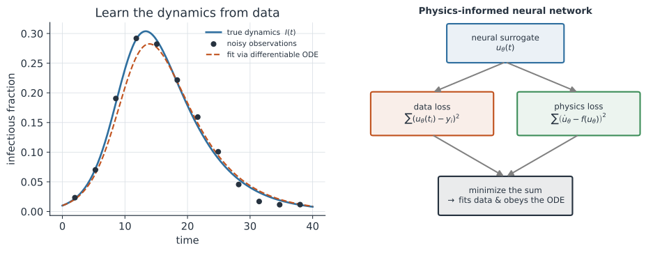
A physics-informed neural network (PINN) attacks the same marriage from the other side. Rather than a network inside the ODE, the network is the solution: train a surrogate $u_\theta(t)$ to approximate the state trajectory, and enforce the known equation through the loss, as in the right of the figure. The loss has two terms, $\mathcal{L}(\theta) = \underbrace{\sum_i \bigl(u_\theta(t_i) - y_i\bigr)^2}_{\text{data misfit}} + \lambda \underbrace{\sum_j \bigl(\dot u_\theta(t_j) - f(u_\theta(t_j))\bigr)^2}_{\text{physics residual}},$ where the first term pulls the surrogate through the observed data and the second penalizes any point where the surrogate violates the differential equation $\dot u = f(u)$ — evaluated using autodiff for the time derivative $\dot u_\theta$ . Because the physics residual can be enforced at any time point, needing no data there, a PINN can fit a mechanistic model from sparse, noisy observations and interpolate sensibly in the gaps, and it handles inverse problems (unknown parameters) by treating them as extra variables to optimize.

A worked example#

Take the SIR curve in the figure, generated with $\beta = 0.6$ , $\gamma = 0.2$ , and observed at noisy time points along the epidemic. Fitting means choosing $(\beta,\gamma)$ to minimize the squared error between the solver’s output and the data. Starting from a poor guess, autodiff gives the gradient of that error with respect to $\beta$ and $\gamma$ through the entire integration, and a run of gradient-descent steps walks the parameters back to near their true values — recovering the mechanism, with its interpretable $R_0 = \beta/\gamma$ , rather than an opaque curve fit.

In code#

Python#

Differentiating through the ODE solver is the heart of it. With JAX we integrate SIR, define a data-misfit loss, and let jax.grad recover the rates — the exact machinery a neural ODE uses, here with a mechanistic vector field:

Python

import jax, jax.numpy as jnp
import numpy as np

def step(u, dt, beta, gamma):                 # one explicit Euler step of SIR
    S, I, R = u
    return jnp.array([S - dt * beta * S * I,
                      I + dt * (beta * S * I - gamma * I),
                      R + dt * gamma * I])

def simulate(beta, gamma, n=400, dt=0.1):     # integrate to a trajectory
    def body(u, _):
        u = step(u, dt, beta, gamma)
        return u, u[1]                         # record the infectious fraction
    _, traj = jax.lax.scan(body, jnp.array([0.99, 0.01, 0.0]), None, length=n)
    return traj

true = simulate(0.6, 0.2)                      # synthetic truth
obs_t = np.arange(10, 400, 10)                 # noisy observations of I(t)
rng = np.random.default_rng(0)
y = np.asarray(true)[obs_t] + rng.normal(0, 0.005, obs_t.size)

def loss(logp):                                # fit in log-space to keep rates > 0
    p = jnp.exp(logp)
    traj = simulate(p[0], p[1])
    return jnp.mean((traj[jnp.array(obs_t)] - jnp.asarray(y)) ** 2)

grad = jax.jit(jax.grad(loss))                  # gradient *through the ODE solver*
logp, m, v = jnp.log(jnp.array([0.3, 0.1])), jnp.zeros(2), jnp.zeros(2)
for t in range(1, 4001):                        # Adam descent from a poor guess
    g = grad(logp)
    m, v = 0.9 * m + 0.1 * g, 0.999 * v + 0.001 * g * g
    logp = logp - 0.05 * (m / (1 - 0.9 ** t)) / (jnp.sqrt(v / (1 - 0.999 ** t)) + 1e-8)
p = np.exp(np.asarray(logp))
print(f"recovered beta={p[0]:.3f}, gamma={p[1]:.3f} (true 0.600, 0.200)")
print(f"recovered R0={p[0] / p[1]:.2f} (true 3.00)")

recovered beta=0.599, gamma=0.201 (true 0.600, 0.200)
recovered R0=2.98 (true 3.00)

A true neural ODE makes the vector field itself a network and backpropagates through the solver with torchdiffeq — here it learns the dynamics of a logistic epidemic curve from scratch:

Python

import torch, torch.nn as nn
from torchdiffeq import odeint                 # differentiable ODE integration
torch.manual_seed(0)

t = torch.linspace(0, 10, 50)
target = 1 / (1 + torch.exp(-(t - 5)))          # a logistic trajectory to learn

class ODEFunc(nn.Module):                        # dy/dt = f_theta(y): the field IS a net
    def __init__(self):
        super().__init__()
        self.net = nn.Sequential(nn.Linear(1, 32), nn.Tanh(), nn.Linear(32, 1))
    def forward(self, t, y):
        return self.net(y)

func = ODEFunc()
opt = torch.optim.Adam(func.parameters(), lr=0.01)
y0 = target[:1].reshape(1, 1)
for _ in range(300):                             # backprop through the ODE solver
    opt.zero_grad()
    pred = odeint(func, y0, t).reshape(-1)
    loss = ((pred - target) ** 2).mean()
    loss.backward(); opt.step()
print(f"neural ODE fit to the trajectory: final MSE {loss.item():.4f}")

neural ODE fit to the trajectory: final MSE 0.0101

A universal differential equation keeps the known SIR terms and adds a small correction = nn.Sequential(...) network inside the field for the unknown part; the training loop is identical.

R#

# deSolve integrates the ODE; a differentiable route uses torch for R.
library(deSolve)
sir <- function(t, u, p) list(c(-p["beta"] * u["S"] * u["I"],
                                 p["beta"] * u["S"] * u["I"] - p["gamma"] * u["I"],
                                 p["gamma"] * u["I"]))
out <- ode(c(S = 0.99, I = 0.01, R = 0), times = seq(0, 40, 0.1), sir,
           c(beta = 0.6, gamma = 0.2))

Julia#

Julia

# Julia's SciML stack (DifferentialEquations + SciMLSensitivity) is the reference
# implementation for neural ODEs and universal differential equations.
using DifferentialEquations, SciMLSensitivity, Optimization
function sir!(du, u, p, t)
    du[1] = -p[1] * u[1] * u[2]
    du[2] =  p[1] * u[1] * u[2] - p[2] * u[2]
    du[3] =  p[2] * u[2]
end
prob = ODEProblem(sir!, [0.99, 0.01, 0.0], (0.0, 40.0), [0.6, 0.2])
# fit p by differentiating solve(prob) through the adjoint method

Why it matters#

Scientific machine learning is the natural home for machine learning in infectious-disease modelling, because the field already has good mechanism and scarce, noisy data — exactly the regime where a pure black box overfits and fails to extrapolate. Differentiable simulation makes fitting compartmental and renewal models to data fast and gradient-based, even with many parameters. Universal differential equations let data reveal the unknown pieces — a time-varying transmission rate, a behavioural feedback, a missing route — while keeping the trusted structure and its interpretable quantities like $R_0$ . Physics-informed networks fit and interpolate mechanistic models from sparse observations and solve inverse problems in one framework. Across all three the payoff is the same: models that respect what we know, learn what we do not, and — unlike a black box — still tell a mechanistic story a public-health decision can rest on.