Species Distribution Models: Presence–Absence Data

When a survey visits chosen sites and records the species as present or absent at each, the modelling gets both easier and more honest than the presence-only case. Now there are real zeros, so occurrence can be modelled as a probability, the absolute prevalence is identifiable, and the model can be validated against the absences it was fit to predict. This is the natural setting for a trap grid, a systematic vector survey, or a designed field campaign.

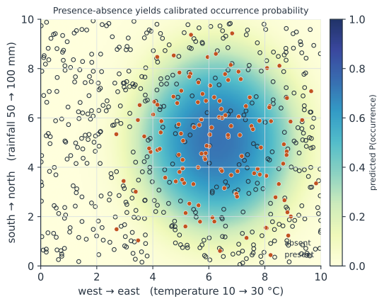
Figure 1. Predicted probability of occurrence across the landscape (shaded) from a logistic model, with survey sites overlaid: filled points where the species was found, open points where it was surveyed and absent. Presences concentrate in the high-probability core; absences dominate the unsuitable margins.

Occurrence as a probability#

With a binary outcome $y_i \in \{0,1\}$ at surveyed site $i$ with environment $z_i$ , the standard model is logistic regression:

$\Pr(y_i = 1) = \operatorname{logit}^{-1}\!\big(\alpha + \beta^\top z_i\big).$

Unlike the presence-only case, the intercept $\alpha$ is now identifiable — it sets the overall occupancy rate — because the absences carry the information about how often the species is not there. The response is often made flexible with quadratic terms or splines (a GAM), or replaced entirely by machine-learning learners — boosted regression trees and random forests are standard in the SDM literature — but the logistic GLM is the interpretable baseline and the one to understand first.

Detection is not occupancy#

A recorded absence is only an apparent absence: the species may be present but undetected. If detection is imperfect and you ignore it, occupancy is underestimated and any covariate that also affects detection is confounded. When repeat visits to each site are available, an occupancy model separates the probability a site is occupied from the probability of detecting the species given occupancy — the same logic as the detection-probability problem for diagnostics, lifted to space.

Evaluating the model#

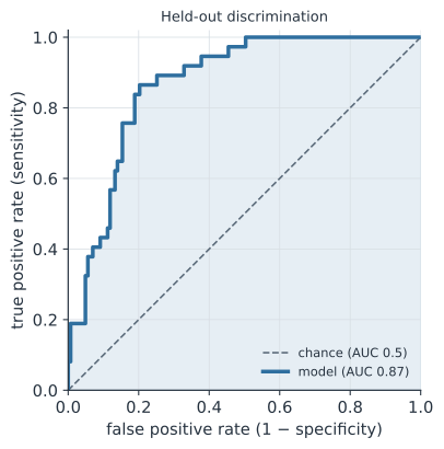
Because there are absences, the model can be scored on how well it discriminates occupied from empty sites. The standard summary is the AUC — the area under the ROC curve, the probability the model ranks a random presence above a random absence (0.5 is chance, 1.0 is perfect). Evaluate it on held-out data, never the training sites, or it is optimistic. Discrimination is not everything: also check calibration (do sites predicted at 30% actually host the species ~30% of the time) before trusting the predicted probabilities as risk.

A worked example#

We survey 600 sites, record presence/absence under a unimodal niche with unmodelled noise, fit a logistic model on a training split, and evaluate on the rest (Figure 2).

Figure 2. The ROC curve for the held-out survey sites; the area under it (AUC ≈ 0.87) is the probability the model ranks a random occupied site above a random empty one. The diagonal is chance.

Python

import numpy as np
from sklearn.linear_model import LogisticRegression
from sklearn.metrics import roc_auc_score

rng = np.random.default_rng(3)
temp = lambda x: 10 + 2.0 * x
rain = lambda y: 50 + 5.0 * y
t_opt, t_w, r_opt, r_w = 22.0, 4.0, 75.0, 12.0

S = 600
sites = rng.uniform(0, 10, size=(S, 2))
niche = -(((temp(sites[:, 0]) - t_opt) ** 2) / (2 * t_w**2)
          + ((rain(sites[:, 1]) - r_opt) ** 2) / (2 * r_w**2))
eta = 1.2 + 2.2 * niche + rng.normal(0, 0.8, S)     # unmodelled site noise
y = (rng.uniform(size=S) < 1 / (1 + np.exp(-eta))).astype(int)

def feats(P):
    t, r = temp(P[:, 0]), rain(P[:, 1])
    return np.column_stack([t, t**2, r, r**2])

X = feats(sites)
Xs = (X - X.mean(0)) / X.std(0)
idx = rng.permutation(S)
tr, te = idx[:420], idx[420:]                       # 70/30 train/test split
m = LogisticRegression(C=1e6, max_iter=5000).fit(Xs[tr], y[tr])

b = m.coef_[0] / X.std(0)
print(f"prevalence (occupied fraction) {y.mean():.2f}")
print(f"held-out AUC {roc_auc_score(y[te], m.predict_proba(Xs[te])[:, 1]):.3f}")
print(f"recovered temp optimum {-b[0] / (2 * b[1]):.1f}  (true {t_opt})")

prevalence (occupied fraction) 0.21
held-out AUC 0.869
recovered temp optimum 22.9  (true 22.0)

In code#

R#

fit <- glm(present ~ poly(temp, 2) + poly(rain, 2), family = binomial, data = sites)
# richer alternatives common in SDMs:
#   mgcv::gam(present ~ s(temp) + s(rain), family = binomial)   # smooth GAM
#   dismo::gbm.step(...)   # boosted regression trees
pROC::auc(test$present, predict(fit, test, type = "response"))  # held-out AUC

Julia#

Julia

using GLM, DataFrames
fit = glm(@formula(present ~ temp + temp^2 + rain + rain^2), sites, Binomial())
# predict(fit, test) gives occurrence probabilities to score against held-out y

Why it matters#

Presence–absence surveys are the gold standard for mapping where a vector or reservoir actually is: entomological trap grids for Aedes and Anopheles, rodent-trapping transects for reservoir hosts, sentinel-site networks. Because they carry true zeros, they yield calibrated probabilities of occurrence — the quantity that feeds a risk map or a vectorial-capacity calculation — and they can be validated honestly against held-out sites. The main trap is treating an apparent absence as a true one: where detection is imperfect, an occupancy model, not a plain GLM, is what keeps the map from underestimating the range.