Burst Size, Latent Period, and Mutation at the Cellular Scale
The same population dynamics that govern how microbes and their hosts interact also play out one scale down, inside a single infected cell. Zoom in from the host to that cell and a virus faces a small number of decisions, each with a mathematical consequence. How long should it commandeer the cell before releasing progeny — its latent period? How many virions should it build in that time — its burst size? And how faithfully should it copy its genome — its mutation rate? Perfect copying would be a trap: some level of variation is itself an advantage, the raw material that lets the virus evolve and adapt to immunity and drugs. These three are the virus’s cellular life-history traits, and they are coupled rather than independent: a longer latent period buys a larger burst, a larger burst is a larger draw from sequence space, and the fidelity of copying sets how much of that draw is mutant. This page works through the math that links them, at the level of the cell, following the viral-ecology tradition that Joshua Weitz synthesized in Quantitative Viral Ecology and that goes back to the phage physiologists.
The cellular parameters#
The within-host models track target cells, infected cells, and free virus with rate constants; here we name the per-cell quantities those rates encode.
| Symbol | Name | Meaning |
|---|---|---|
| eclipse period | time from infection until the first progeny virion is assembled | |
| latent period | time from infection until progeny release (lysis, or onset of budding); | |
| production rate | virions assembled per unit time during the productive phase | |
| burst size | total progeny virions released by one infected cell | |
| infected-cell death rate | is the mean productive lifespan of a cell | |
| virion clearance rate | rate at which a free virion is lost (decay, clearance) | |
| adsorption hazard | rate a free virion successfully attaches to a target cell | |
| per-site mutation rate | probability a given base is miscopied per replication | |
| genomic mutation rate | expected new mutations per genome per replication ( = genome length) |
Two things separate viruses at this scale. Lytic viruses — the bacteriophage archetype — accumulate progeny internally and release them in one burst when the cell lyses, so and are tightly coupled. Budding viruses (influenza, HIV, coronaviruses) release virions continuously over the cell’s lifespan, so the “burst” is a lifetime yield rather than a single event — a distinction that turns out to matter for stochastic fate but not for mean dynamics. The split is cleaner in theory than in cells: careful single-cell work now argues that nonlytic egress dominates the animal-virus world, with even textbook “lytic” nonenveloped viruses such as poliovirus exported largely in membrane vesicles hours before the cell dies — so read the lytic burst as a mathematical idealization (exact for phages, approximate for animal viruses) rather than a literal account of how progeny leave the cell.
Burst size is accumulated over the latent period#
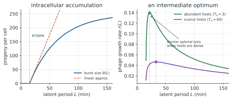
Nothing is released during the eclipse; after it, progeny accumulate at rate , so to a first approximation the burst grows linearly with how long the virus waits to lyse,
In reality the curve in Figure 1 bends over: as the cell’s ribosomes, nucleotides, and membrane are exhausted, production saturates toward a ceiling , well described by . Single-cell measurements confirm both the rising-then-saturating shape and something the deterministic picture hides: burst size is wildly heterogeneous from cell to cell. For influenza A, single infected cells span to virions, with ~10% of cells (“super-producers”) making 40–60% of all progeny; HSV-1 progeny from single keratinocytes span three orders of magnitude for the same reason. The linear law (1) is the mean of a very broad distribution — a cell-scale echo of the superspreading heterogeneity seen between hosts.
The cellular reproduction number#
The burst is only worth what its virions go on to infect. A released virion is in a race: it is cleared at hazard and adsorbs to a fresh target cell at hazard , so the probability it wins the race and starts a new infection is
Multiplying the number of tickets by the chance each one wins gives the cellular reproduction number — how many new infected cells one infected cell produces:
This is exactly the within-host in disguise. In the standard target-cell model an infected cell produces virus at rate for a mean lifespan , so its lifetime burst is ; each virion, in the small-adsorption limit , infects with probability . Substituting into (3) recovers the familiar
which is the formula derived from the next-generation matrix of the ODE model. The lesson is that at the cellular scale is nothing but burst size times per-virion establishment probability — every route to it is a way of writing .
Continuous versus burst production: same mean, different fate#
Here is a fact that surprises people the first time. A budding virus that trickles out virus at rate over a lifespan , and a lytic virus that releases the whole burst at the instant of lysis, produce identical deterministic dynamics — the ODEs cannot tell them apart, because only the lifetime total enters the mean-field equations. But Pearson and colleagues showed that stochastically they differ, and the difference lives in the offspring distribution of a single infected cell.
Model each cell as producing a random number of successful secondary infections; by branching-process theory the probability a lineage started by one infected cell dies out is the smallest root of , where is the probability generating function.
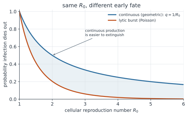
Continuous production, exponential lifespan. A cell emits successful infections as a Poisson process (rate ) while it lives, and dies at rate . Racing production against death gives a geometric offspring count with mean , PGF with , and a clean closed-form extinction probability:
Lytic burst. A cell releases a fixed virions at once, each independently establishing with probability , so , which for large and small is with PGF and extinction probability solving
Both have the same mean , but the geometric distribution is over-dispersed (variance ) while the Poisson burst is not (variance ). More variance means more mass on “zero offspring,” so the continuous mode is always easier to extinguish: for every , as Figure 2 shows.
Real cells sit between these extremes. With an eclipse phase and a staged infectious period, the reproduction number of a single cell is a negative binomial random variable, and the probability of establishment depends on that whole distribution, not just its mean — the same reason dispersion governs outbreak fate between hosts. Both idealizations also assume virions establish independently; when a virus egresses en bloc — many genomes bundled inside one membrane vesicle, transmission turns collective and the multiplicity of infection climbs, a further departure from the single-genome offspring counts above.
The optimal latent period: a marginal-value problem#
Waiting longer to lyse trades higher burst for slower turnover — the phage version of “a bird in the hand versus two in the bush.” The classic treatment casts it as optimal foraging via the marginal value theorem: the cell is a patch, progeny are the resource, and lysis is the decision to leave. Consider a phage growing in a well-mixed host population where a free phage takes a mean search time to find and adsorb a host (density ). Each infection cycle multiplies the phage by over a generation of length , so the long-run population growth rate is
Maximising (6) — setting — gives the optimality condition
the marginal value theorem in one line: lyse at the moment the marginal rate of building new progeny falls to the average rate of return of the whole cycle. Because is concave (it saturates), (6) has a single interior peak — an intermediate latent period is optimal, exactly as Wang built an isogenic λ-phage panel to confirm and Kannoly verified in continuous culture. The comparative statics fall straight out of (7): when hosts are abundant ( small) the cost of a long wait is high, so the optimum shifts to shorter lysis times (right panel of Figure 1), the prediction Abedon confirmed experimentally by enriching for short-latent-period mutants at high bacterial density.
Notice how flat the fitness curve is near its peak in Figure 1. A broad optimum means selection on lysis timing is weak once you are close, which is why real latent periods are variable and why cell-to-cell noise in lysis timing both persists and biases the classic one-step growth-curve estimate of downward.
Mutation: burst size is a lottery for variation#
Every one of the progeny is a fresh copy of the genome, and copying is imperfect. If a specific escape or resistance mutation arises at per-site rate , then the number of progeny in a single burst carrying it is , so the expected number of mutant progeny per cell is simply the product
Burst size and mutation rate enter only through — the per-cell mutational output — so a large burst is a large draw from sequence space even when fidelity is high (Figure 3). Counting any mutation rather than one specific site, each progeny genome carries a number of new mutations, so the cell emits mutant progeny per burst; for an RNA virus with that is a mutant in roughly two of every five virions produced.
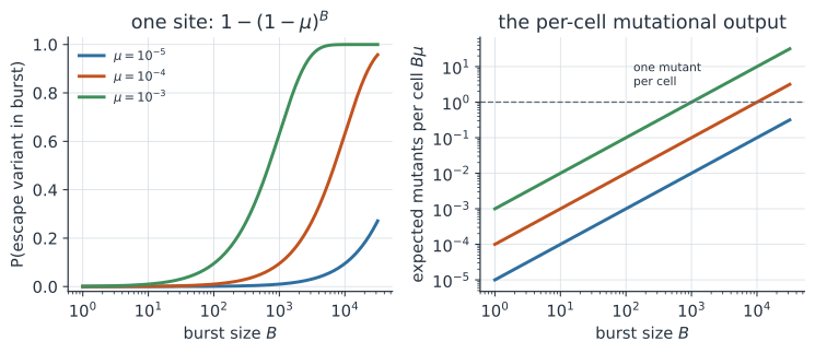
Two consequences follow. First, (8) is a mean; because a mutation that arises early in the intracellular replication tree is amplified into many progeny, the distribution of mutants per burst is heavy-tailed and Luria–Delbrück-like, with rare “jackpot” cells — the within-cell analogue of the jackpot lineages that dominate mutation-supply variance. Second, the total supply of any variant across an infection is , so high-burst, high-mutation viruses explore genotype space fastest. Push the genomic rate up far enough and this becomes a liability: past the error threshold the population can no longer maintain its master sequence, the principle behind lethal mutagenesis as an antiviral strategy. Burst size and mutation rate are the numerator and the per-copy risk of the same lottery.
A worked example#
Take a lytic virus with eclipse min, saturating yield , time-scale min, so at a 60-minute latent period virions. Suppose a released virion adsorbs at hazard and is cleared at , so and the cellular — a vigorous infection well above threshold. Near the establishment threshold, though, the production mode matters: at a continuously-shedding cell’s lineage dies out with probability , whereas an equal-mean lytic burst dies out only with — the budding virus is more than twice as likely to fizzle from a single seeding cell. On mutation, with per-site the 148-virion burst throws a given point mutant with probability ; a super-producer cell making raises that to , and its expected genome-wide mutant output () is mutant progeny from that one cell. The rare high-burst cells are doing most of the evolving.
Eleven viruses across the cellular parameter space#
The equations above are a common currency, so the most useful thing to do with them is compare real viruses that solve the cellular problem in very different ways. Ten of the eleven below are RNA viruses; the last, variola (smallpox), is a large double-stranded DNA poxvirus — together they span the parameter space along all three axes at once, burst size, mutation rate, and the length of the production window. Rather than give each virus its own colour, Figure 4 colours them by life-history strategy — how they exploit the cell — so the picture stays legible as viruses are added, with individuals read from the labels and this table. Four strategies cover them: a lytic burst at cell death (poliovirus, and variola’s DNA factories are freed much the same way); acute budding, continuous release while the cell dies (HIV, influenza, dengue); syncytial release, budding but fusing the cell into a dying syncytium (the paramyxo- and pneumoviruses measles, mumps, RSV, and the henipaviruses Nipah and Hendra); and persistent, non-cytopathic release with the window held open (hantavirus). Those differences in how, how many, and how fast explain a great deal of their epidemiology. (The table lists one virus per row; the same seven traits are the columns.)
| Virus | Genome | Production mode | Infected-cell fate | Eclipse | Burst size | Per-site mutation | Evolutionary signature |
|---|---|---|---|---|---|---|---|
| HIV-1 | retrovirus, +ssRNA → DNA, ~9.7 kb | budding, continuous | dies in ~1–2 days (cytopathic + CTL) | ~18–24 h | ~– total, ~1 in – infectious | ~ (RT); ~ in vivo via APOBEC | quasispecies, rapid drug/immune escape |
| Influenza A | −ssRNA, 8 segments, ~13.5 kb | budding, ~continuous | dies in ~1 day (cytopathic) | ~6 h | ~– (single-cell mean ~350–700) | ~– (2–3 per genome) | antigenic drift + segment reassortment |
| Hantavirus | −ssRNA, 3 segments, ~12 kb | budding, continuous | survives — non-cytopathic, persistent | ~1–3 days | low–moderate, IFN-limited, sustained | RNA-range but constrained; low diversity | host codivergence, spillover dead-end |
| Poliovirus | +ssRNA, non-segmented, ~7.5 kb | lytic burst (much egress nonlytic, in EVs) | lyses by ~6–8 h, but egress precedes it | ~2–3 h | ~– per cell | ~ (RdRp, no proofreading) | high diversity but 3 fixed serotypes; vaccine-derived reversion |
| Measles | −ssRNA, non-segmented, ~15.9 kb | budding, syncytial | fuses into dying syncytia over ~2–3 days | ~12–24 h | low–moderate (~–) | ~ (RNA-range) | monotypic — one serotype, antigenically stable |
| Mumps | −ssRNA, non-segmented, ~15.4 kb | budding, syncytial | fuses into dying syncytia (~2–3 days) | ~12–24 h | low–moderate (~–) | ~– (RNA-range) | 12 genotypes; vaccine-era outbreaks (waning + escape) |
| RSV | −ssRNA, non-segmented, ~15.2 kb | budding, syncytial | fuses into dying syncytia (~2–3 days) | ~10–12 h | low; high particle-to-PFU ratio | ~ (RNA-range) | A/B subgroups; variable G, conserved F |
| Nipah | −ssRNA, non-segmented, ~18.2 kb | budding, syncytial | fuses into dying syncytia (~2–3 days) | ~12–24 h | moderate (~–) | ~ (RNA-range, conserved) | bat reservoir; BSL-4 spillover, high CFR |
| Hendra | −ssRNA, non-segmented, ~18.2 kb | budding, syncytial | fuses into dying syncytia (~2–3 days) | ~12–24 h | moderate (~–) | ~ (RNA-range, conserved) | flying-fox reservoir; horse-mediated spillover |
| Dengue | +ssRNA, non-segmented, ~10.7 kb | budding (secretory) | dies by apoptosis (~2–3 days) | ~12–24 h | ~– | ~– (RdRp) | 4 serotypes; cross-serotype ADE |
| Variola | dsDNA, ~186 kb | on lysis (MV) plus budding (EV) | dies (cytopathic, ~1–2 days) | ~6–12 h | ~– | ~ (proofreading DNA pol) | genetically stable; eradicated by one vaccine |
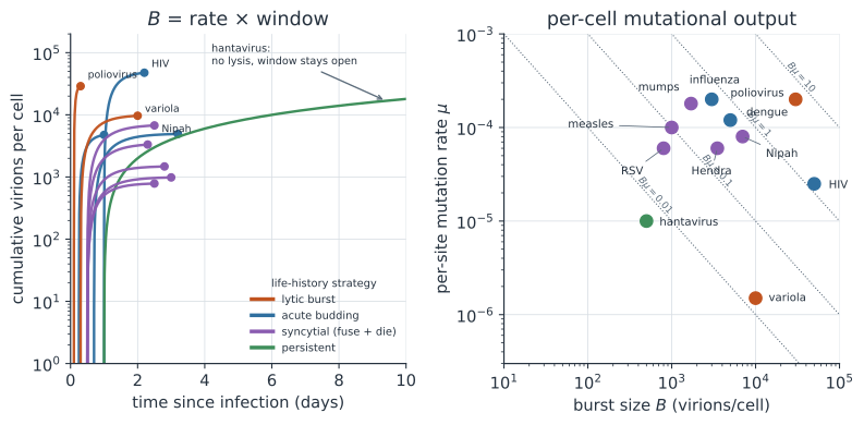
The production window, not the burst rate, is what hantavirus changes. Recall that lifetime burst is production rate times production window, and for a lytic or cytopathic virus the window is the cell’s lifespan . Influenza and HIV both kill the cell — influenza fast, HIV a little slower — so their yield is capped by how long the cell survives (left panel of Figure 4); HIV’s in-vivo per-cell yield is ~– virions but only about one in a few hundred is infectious, so the effective burst that enters is far smaller than the RNA count. Poliovirus is the same accounting compressed into hours: it packages – virions in a cell that lasts only about 6–8 h — a very high production rate over a very short window, the steep early climb in the left panel. Measles, RSV, and dengue sit in between: all three bud yet still kill the cell — measles and RSV by fusing it into dying syncytia, dengue by driving it to apoptosis — so their windows are bounded like influenza’s while their production rates stay modest, which is why their curves in the left panel plateau at intermediate yields. Hantaviruses are the striking case: they replicate in vascular endothelial cells with no cytopathic effect and establish persistent infection, so and the window is set not by lysis but by interferon. In human cells IFN-β switches on after a few days and production falls off; in the natural rodent reservoir the antiviral response is never triggered, the window stays open indefinitely, and the animal remains a lifelong low-level shedder. The same accounting, with the death term turned off, is the whole difference between an acute and a persistent infection.
Production mode sorts their stochastic fate. The nine budding viruses release virus continuously rather than in a synchronized burst, so the offspring distribution of a single infected cell is closer to the over-dispersed geometric of (4) than to the Poisson of (5), with extinction probability near . This is why single-cell seeding is fragile even for a fit virus, and it is consistent with the very narrow transmission bottleneck of HIV, where a productive infection is usually founded by a single transmitted variant despite the donor carrying a diverse swarm. Poliovirus makes the mechanism visible: because it releases its whole burst at lysis, a single cell’s successful-offspring count is Poisson (5) rather than geometric, so at the same mean a lone poliovirus-infected cell is meaningfully harder to extinguish than any of the budding nine — the burst-versus-continuous gap of Figure 2, now a difference between real viruses. Variola sits on the same side of that gap: much of its progeny is freed when the cell lyses rather than trickled out over a lifetime, so its single-cell offspring count leans burst-like too, a Poisson-ish case set against the geometric budders. Both “burst” cases carry the caveat flagged earlier, though: poliovirus and the poxviruses in fact export a large share of their yield nonlytically, in vesicles and often en bloc, so their true offspring statistics fall between the Poisson and geometric extremes rather than sitting cleanly at the burst end — the diagram treats them as the idealized burst case to make the mechanism legible, not as a literal claim that they only release at lysis.
Mutational output separates the fast evolvers from the stable ones. The per-cell mutational output is , and the right panel of Figure 4 places all eleven viruses on the – plane against diagonals of constant . Influenza sits high on — ~ per site, 2–3 mutations per genome copied — which, multiplied over large bursts, is the raw material of antigenic drift, compounded by reassortment of its eight segments. HIV’s reverse transcriptase runs at the canonical RNA-virus rate ~, but its enormous within-host replication and APOBEC-driven hypermutation push the in-vivo rate to ~ — the highest measured for any biological entity — which is why drug resistance is essentially pre-existing in every patient. Hantaviruses sit in the low corner: their persistent, low-turnover replication accumulates change slowly, and their tight codivergence with rodent hosts leaves them genetically stable and host-restricted — part of why human infections are typically epidemiological dead ends rather than the start of sustained human-to-human chains. Poliovirus and measles are the cautionary corner: poliovirus has the highest per-cell mutational output of the eleven (, a large burst copied at RdRp fidelity) and measles carries an ordinary RNA-range , yet both are antigenically almost frozen — poliovirus in three fixed serotypes, measles as a single serotype the 1960s vaccine still matches — because their capsid and glycoprotein structures are functionally constrained, so most of that variation is either lethal or invisible to immunity. The syncytial paramyxoviruses fan out around measles precisely because that constraint is not absolute: mumps, its close relative, carries near-identical and yet its surface proteins are not as locked down, so the same mutational supply has produced twelve genotypes and repeated vaccine-era outbreaks in highly immunised populations; the henipaviruses Nipah and Hendra sit the other way, held genetically stable by strong purifying selection and codivergence with their fruit-bat reservoirs, so their menace is spillover and a high case-fatality rate, not antigenic escape — a reminder that whether variation becomes useful is a property of the protein and its selective regime, not of . RSV and dengue occupy the same middle ground, carrying just enough usable antigenic variation to matter epidemiologically: RSV splits into A and B subgroups on its variable G protein while its fusion protein stays conserved, and dengue’s four serotypes are the substrate for antibody-dependent enhancement, where prior immunity to one serotype worsens infection by another. Variola is the opposite extreme in fidelity, and the one point that leaves the RNA cloud entirely: its proofreading DNA polymerase holds the per-site rate near , an order of magnitude below any RNA virus here, so despite a burst of its per-cell mutational output stays low (, down in the corner with hantavirus) — the molecular reason smallpox stayed a single, antigenically fixed target for centuries and could be driven to global eradication with one vaccine. They are the standing reminder that sets the supply of variants, not whether any of them can become useful: read through that product, the same quantity that sets a phage’s supply of escape mutants explains why influenza and HIV are moving targets, why hantavirus (little variation) and poliovirus, measles, and the henipaviruses (plenty of variation, nowhere to go) are not, why mumps, RSV, and dengue land in between, and why variola — its output low and its structure constrained — was the one virus a vaccine could corner into extinction.
In code#
We reproduce all four scenarios: the cellular from a burst, the continuous-versus-burst extinction gap, the optimal latent period, and the mutational output per burst.
R#
eclipse <- 15; Bmax <- 250; kappa <- 50
burst <- function(L) ifelse(L > eclipse, Bmax * (1 - exp(-(L - eclipse) / kappa)), 0)

# cellular R0 = B * rho
beta_x0 <- 0.8; u <- 4
rho <- beta_x0 / (beta_x0 + u)
R0  <- burst(60) * rho
cat(sprintf("B(60) = %.0f, rho = %.3f, cellular R0 = %.1f\n", burst(60), rho, R0))

# continuous (geometric) vs burst (Poisson) extinction at a shared mean R0
q_burst <- function(R) uniroot(function(q) exp(R * (q - 1)) - q, c(1e-9, 1 - 1e-9))$root
for (R in c(1.5, 2, 3))
  cat(sprintf("R0=%.1f: extinction continuous %.3f vs burst %.3f\n", R, 1 / R, q_burst(R)))

# optimal latent period maximising r(L) = ln B(L) / (Ta + L)
grid <- seq(eclipse + 0.5, 160, length.out = 4000)
for (Ta in c(3, 60)) {
  Lstar <- grid[which.max(log(burst(grid)) / (Ta + grid))]
  cat(sprintf("Ta=%2.0f: optimal L = %.1f min, burst = %.0f\n", Ta, Lstar, burst(Lstar)))
}

# mutation: expected mutants and escape probability per burst
mu <- 3e-5; U <- 0.5                            # per-site rate; per-genome rate
for (B in c(30, 148, 5000))
  cat(sprintf("B=%5d: E[site mutants]=%.3f, P(escape)=%.3f, E[mutant progeny]=%.0f\n",
              B, B * mu, 1 - (1 - mu)^B, B * (1 - exp(-U))))
Python#
import numpy as np
from scipy.optimize import brentq

# 1. Intracellular accumulation and the cellular reproduction number R0 = B * rho
eclipse, Bmax, kappa = 15.0, 250.0, 50.0
burst = lambda L: np.where(L > eclipse, Bmax * (1 - np.exp(-(L - eclipse) / kappa)), 0.0)
beta_x0, u = 0.8, 4.0                      # per-virion adsorption vs clearance hazards
rho = beta_x0 / (beta_x0 + u)              # prob a released virion infects a new cell
B60 = float(burst(60.0))
print(f"B(60 min) = {B60:.0f} virions, rho = {rho:.3f}, cellular R0 = {B60 * rho:.1f}")

# 2. Same mean R0, two production modes -> different extinction (near threshold)
for R in (1.5, 2.0, 3.0):
    q_burst = brentq(lambda q: np.exp(R * (q - 1)) - q, 1e-9, 1 - 1e-9)
    print(f"R0={R}: extinction  continuous {1/R:.3f}  vs  burst {q_burst:.3f}")

# 3. Optimal latent period maximises r(L) = ln B(L) / (T_a + L)
grid = np.linspace(eclipse + 0.5, 160, 4000)
for Ta in (3.0, 60.0):
    Lstar = grid[np.argmax(np.log(burst(grid)) / (Ta + grid))]
    print(f"T_a={Ta:4.0f}: optimal L = {Lstar:.1f} min, burst = {burst(Lstar):.0f}")

# 4. Mutation: expected mutants and escape probability per burst
mu, U = 3e-5, 0.5                          # per-site rate; per-genome rate (RNA scale)
for B in (30, 148, 5000):
    print(f"B={B:5d}: E[site mutants]={B*mu:.3f}, "
          f"P(escape)={1-(1-mu)**B:.3f}, E[mutant progeny]={B*(1-np.exp(-U)):.0f}")
B(60 min) = 148 virions, rho = 0.167, cellular R0 = 24.7
R0=1.5: extinction  continuous 0.667  vs  burst 0.417
R0=2.0: extinction  continuous 0.500  vs  burst 0.203
R0=3.0: extinction  continuous 0.333  vs  burst 0.060
T_a=   3: optimal L = 21.7 min, burst = 31
T_a=  60: optimal L = 32.9 min, burst = 75
B=   30: E[site mutants]=0.001, P(escape)=0.001, E[mutant progeny]=12
B=  148: E[site mutants]=0.004, P(escape)=0.004, E[mutant progeny]=58
B= 5000: E[site mutants]=0.150, P(escape)=0.139, E[mutant progeny]=1967
Julia#
using Roots

eclipse, Bmax, kappa = 15.0, 250.0, 50.0
burst(L) = L > eclipse ? Bmax * (1 - exp(-(L - eclipse) / kappa)) : 0.0

beta_x0, u = 0.8, 4.0
rho = beta_x0 / (beta_x0 + u)
println("B(60) = $(round(burst(60); digits=0)), cellular R0 = $(round(burst(60)*rho; digits=1))")

# continuous (geometric) vs lytic-burst (Poisson) extinction
for R in (1.5, 2.0, 3.0)
    qb = find_zero(q -> exp(R * (q - 1)) - q, (1e-9, 1 - 1e-9))
    println("R0=$R: extinction continuous $(round(1/R; digits=3)) vs burst $(round(qb; digits=3))")
end

# optimal latent period
grid = range(eclipse + 0.5, 160; length = 4000)
for Ta in (3.0, 60.0)
    Lstar = grid[argmax(log.(burst.(grid)) ./ (Ta .+ grid))]
    println("Ta=$Ta: optimal L = $(round(Lstar; digits=1)) min, burst = $(round(burst(Lstar); digits=0))")
end

# mutation: expected mutants and escape probability per burst
mu, U = 3e-5, 0.5                            # per-site rate; per-genome rate
for B in (30, 148, 5000)
    println("B=$B: E[site mutants]=$(round(B*mu; digits=3)), " *
            "P(escape)=$(round(1 - (1 - mu)^B; digits=3)), " *
            "E[mutant progeny]=$(round(B * (1 - exp(-U)); digits=0))")
end
Why it matters#
The three cellular traits on this page are the microscopic origins of the macroscopic quantities the rest of infectious-disease modelling takes as given. Burst size and per-virion establishment set the within-host that decides whether an infection takes hold; the production mode and the eclipse phase set the stochastic extinction probability that decides whether a single exposed cell — or a single spilled-over host — starts anything at all. The latent-period optimum is a life-history trade-off that natural selection actually solves, and the same curve that governs a phage’s optimal lysis time governs how a within-host virus tunes its replication against immune clearance. And the product is the engine of viral evolution: it is the per-cell supply of the variation that becomes drug resistance, immune escape, and — pushed too far by design — the error catastrophe that antiviral mutagens exploit. Reading a virus at the scale of the cell turns “how fast, how many, how sloppy” into equations that connect all the way up to the epidemic.
Related#
- Within-Host Dynamics and the Immune Response — the target-cell ODEs whose rate constants these per-cell traits encode
- Branching Processes — the extinction-probability machinery used here
- Superspreading and Transmission Heterogeneity — the between-host analogue of cell-to-cell burst heterogeneity
- Quasispecies and the Error Threshold — where the mutational-output story leads
- Resistance Evolution and Lethal Mutagenesis — pushing past the edge of viability
- The Evolution of Virulence — life-history trade-offs one scale up
- Stochastic Epidemics and the Gillespie Algorithm — simulating the noisy early dynamics
- The Euler–Lotka Equation — the renewal-equation view of the growth rate
- Quantitative Methods