Dilutions, Titers, and Standard Curves
An assay never hands you a concentration directly. It gives a readout — a count of plaques, the last dilution that still shows an effect, an optical density — and the quantitative work is turning that readout back into “how much was in the sample.” This page collects the two everyday calculations that do it: the serial-dilution titer used throughout serology and virology, and the standard-curve interpolation used for continuous readouts like an ELISA optical density.
Serial dilutions and the dilution factor#
A serial dilution repeatedly dilutes a sample by a fixed factor — two-fold and ten-fold are the usual choices — so the concentration in tube falls geometrically:
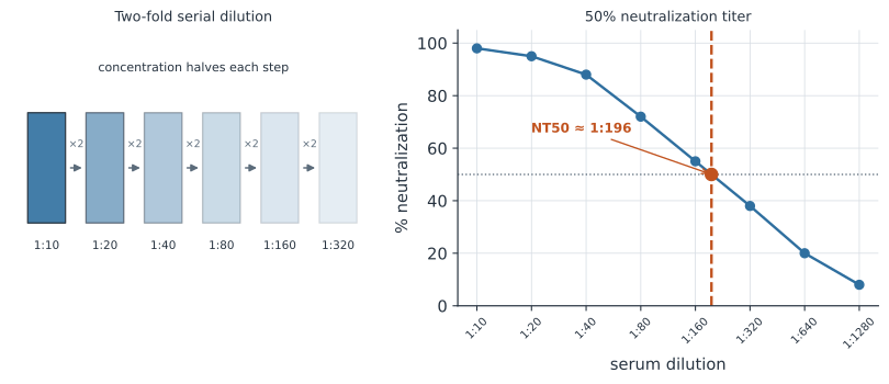
where is the dilution factor. Ten-fold steps span orders of magnitude quickly (for counting colonies or plaques); two-fold steps give the finer resolution wanted for a titer (Figure 1).
To recover the original concentration from a countable dilution, undo the dilution and the plated volume. If a plate seeded with a dilution and inoculum grows plaques, the stock titer is
with the count, the dilution fraction, and the plated volume. The same arithmetic gives CFU/mL for bacteria or copies/mL for a spiked qPCR standard.
Endpoint and 50% titers#
For a graded readout — neutralization, hemagglutination inhibition, agglutination — the result is reported as a titer: the reciprocal of a dilution. The simplest is the endpoint titer, the reciprocal of the highest dilution still scoring positive against a cutoff. It is crude, because it can only land on the discrete dilutions actually tested.
A 50% titer is far more stable: the dilution at which the response is half-maximal — NT50 for neutralization, TCID50 or ID50 for infectivity. Because responses are roughly linear in the log of the dilution, you interpolate on the log scale between the two dilutions that bracket 50%:
where and are the log-dilutions and responses on either side of 50%. For strictly all-or-none readouts (each replicate positive or negative), the Spearman–Kärber estimator does the same job for the 50% infectious dose, summing the response proportions across the dilution series.
A worked example: neutralization titer#
A serum is tested in two-fold dilutions and the percent neutralization recorded at each. We recover the plaque titer of the virus stock and the serum’s NT50 by log-linear interpolation.
import numpy as np

# virus stock titer from a plaque count
plaques, dilution, volume = 32, 1e-4, 0.1          # count, dilution, mL plated
titer = plaques / (dilution * volume)
print(f"stock titer = {titer:.2e} PFU/mL")

# serum neutralization: reciprocal dilution and percent neutralized
recip = np.array([10, 20, 40, 80, 160, 320, 640, 1280.0])
pct = np.array([98, 95, 88, 72, 55, 38, 20, 8.0])

lx = np.log2(recip)
i = np.where(pct >= 50)[0][-1]                      # last dilution >= 50%
xstar = lx[i] + (pct[i] - 50) / (pct[i] - pct[i + 1]) * (lx[i + 1] - lx[i])
nt50 = 2**xstar
endpoint = recip[i]                                 # crude endpoint titer
print(f"endpoint titer 1:{endpoint:.0f}   interpolated NT50 1:{nt50:.0f}")
stock titer = 3.20e+06 PFU/mL
endpoint titer 1:160   interpolated NT50 1:196
The interpolated NT50 (about ) sits between the tested dilutions, where the crude endpoint could only report — a real gain in precision for the same plate.
Standard curves: continuous readouts#
When the readout is a continuous signal — an ELISA optical density, a fluorescence — you calibrate against standards of known concentration and read unknowns off the fitted curve. Optical density saturates, so the standard model is the four-parameter logistic (4PL) introduced on the ELISA page:
with bottom , top , EC50 , and Hill slope . Fit it to the standards, then invert it to turn an unknown OD back into a concentration:
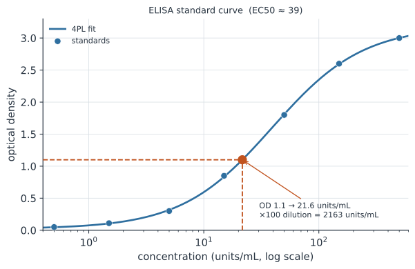
Two practical rules travel with every standard curve (Figure 2):
- Stay inside the dynamic range. Interpolation is only trustworthy between the lowest and highest standards; a sample above saturation must be diluted and re-run.
- Multiply back by the dilution factor. A sample pre-diluted to bring it on-scale reads a concentration smaller than the truth — the interpolated value must be scaled back up.
A worked example: ELISA optical density#
A serum is pre-diluted to land within the assay’s range and read at OD . We fit the 4PL to the standards, invert it, and correct for the dilution.
from scipy.optimize import curve_fit

def fourpl(x, a, d, c, b):
    return d + (a - d) / (1 + (x / c) ** b)

conc = np.array([0.5, 1.5, 5, 15, 50, 150, 500.0])         # standards (units/mL)
od = np.array([0.05, 0.11, 0.30, 0.85, 1.8, 2.6, 3.0])
(a, d, c, b), _ = curve_fit(fourpl, conc, od, p0=[0.03, 3.1, 20, 1.0],
                            maxfev=20000)

od_unknown, dil_factor = 1.10, 100
x = c * ((a - d) / (od_unknown - d) - 1) ** (1 / b)         # invert the 4PL
print(f"EC50 = {c:.1f} units/mL   Hill slope = {b:.2f}")
print(f"OD {od_unknown} -> {x:.1f} units/mL  x{dil_factor} = {x*dil_factor:.0f} units/mL")
EC50 = 39.3 units/mL   Hill slope = 1.10
OD 1.1 -> 21.6 units/mL  x100 = 2163 units/mL
The raw interpolation gives about units/mL; multiplied by the pre-dilution, the reported concentration is roughly units/mL — the number that would be wrong by a hundred-fold if the dilution step were forgotten.
In code#
R#
fourpl <- function(x, a, d, c, b) d + (a - d) / (1 + (x / c)^b)
conc <- c(0.5, 1.5, 5, 15, 50, 150, 500)
od   <- c(0.05, 0.11, 0.30, 0.85, 1.8, 2.6, 3.0)
fit  <- nls(od ~ fourpl(conc, a, d, c, b),
            start = list(a = 0.03, d = 3.1, c = 20, b = 1))
p <- coef(fit)
x <- p["c"] * ((p["a"] - p["d"]) / (1.10 - p["d"]) - 1)^(1 / p["b"])
x * 100          # apply the 1:100 dilution factor
Julia#
using LsqFit
fourpl(x, p) = p[2] .+ (p[1] .- p[2]) ./ (1 .+ (x ./ p[3]) .^ p[4])
conc = [0.5, 1.5, 5, 15, 50, 150, 500.0]
od   = [0.05, 0.11, 0.30, 0.85, 1.8, 2.6, 3.0]
fit = curve_fit(fourpl, conc, od, [0.03, 3.1, 20.0, 1.0])
a, d, c, b = fit.param
x = c * ((a - d) / (1.10 - d) - 1)^(1 / b) * 100     # invert and un-dilute
Multiple plates: one curve per plate#
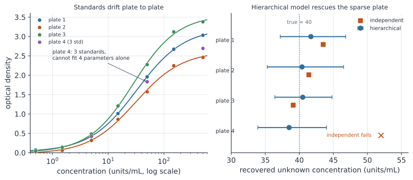
The single curve above calibrates one plate. A real run spans many plates, and absolute OD drifts from plate to plate — reagent age, incubation time, the reader, edge effects — so each plate carries its own standards and is read against its own curve. Sharing one curve across plates is a classic and serious error. But fitting every plate in complete isolation has its own failure mode: a plate with only a few usable standards (a short curve, or dropped wells) cannot pin down all four 4PL parameters on its own.
A Bayesian hierarchical model threads the needle. The curve shape — the Hill slope and the EC50 — is shared across plates (it is the same chemistry), while the plate-specific signal level (the top ) is given a partial-pooling prior, . Each plate keeps its own top, but a plate with sparse standards borrows strength from the others toward the population, instead of failing outright (Figure 3).
import jax.numpy as jnp
from jax import random
import numpyro
import numpyro.distributions as dist
from numpyro.infer import MCMC, NUTS

# four plates; plate 4 has only three standards (a short curve)
rng = np.random.default_rng(0)
a_t, d_pop, c_t, b_t, noise = 0.03, 3.1, 30.0, 1.10, 0.05
tops = d_pop * np.array([1.00, 0.85, 1.15, 0.92])          # plate-to-plate drift
full = np.array([0.5, 1.5, 5, 15, 50, 150, 500.0])
standards = {0: full, 1: full, 2: full, 3: np.array([5, 50, 500.0])}
x_true = 40.0                                              # true unknown, every plate

sx, sp, sy, y_unknown = [], [], [], []
for p in range(4):
    for x in standards[p]:
        sx.append(x); sp.append(p)
        sy.append(fourpl(x, a_t, tops[p], c_t, b_t) + rng.normal(0, noise))
    y_unknown.append(fourpl(x_true, a_t, tops[p], c_t, b_t) + rng.normal(0, noise))
sx, sp, sy, y_unknown = map(np.asarray, (sx, sp, sy, y_unknown))

# independent per-plate fits: plate 4 cannot be fit (3 points, 4 parameters)
indep = []
for p in range(4):
    m = sp == p
    try:
        (a, d, c, b), _ = curve_fit(fourpl, sx[m], sy[m], p0=[0.03, 3.1, 30, 1.0],
                                    maxfev=20000)
        indep.append(c * ((a - d) / (y_unknown[p] - d) - 1) ** (1 / b))
    except (TypeError, RuntimeError):
        indep.append(np.nan)
print("independent recovery (true 40):",
      ", ".join("fails" if np.isnan(v) else f"{v:.1f}" for v in indep))

def hier(sx, sp, sy, yu, P):
    a = numpyro.sample("a", dist.Normal(0.03, 0.05))
    c = numpyro.sample("c", dist.LogNormal(np.log(30), 0.5))    # shared EC50
    b = numpyro.sample("b", dist.LogNormal(0.0, 0.3))           # shared Hill slope
    d_pop = numpyro.sample("d_pop", dist.Normal(3.0, 0.5))
    sig_d = numpyro.sample("sig_d", dist.HalfNormal(0.5))
    sig = numpyro.sample("sig", dist.HalfNormal(0.1))
    with numpyro.plate("plates", P):
        d = numpyro.sample("d", dist.Normal(d_pop, sig_d))      # partial-pooled top
        lx = numpyro.sample("lx", dist.Normal(np.log(30), 1.5))
    x_un = numpyro.deterministic("x_unknown", jnp.exp(lx))
    numpyro.sample("os", dist.Normal(d[sp] + (a - d[sp]) / (1 + (sx / c) ** b), sig),
                   obs=sy)
    numpyro.sample("ou", dist.Normal(d + (a - d) / (1 + (x_un / c) ** b), sig), obs=yu)

mcmc = MCMC(NUTS(hier), num_warmup=1500, num_samples=2000, num_chains=1,
            progress_bar=False)
mcmc.run(random.PRNGKey(0), jnp.array(sx), jnp.array(sp), jnp.array(sy),
         jnp.array(y_unknown), 4)
xu = np.array(mcmc.get_samples()["x_unknown"])
print("hierarchical recovery (true 40):")
for p in range(4):
    lo, hi = np.percentile(xu[:, p], [2.5, 97.5])
    tag = "  <- rescued (3 standards)" if p == 3 else ""
    print(f"  plate {p+1}: {xu[:, p].mean():.1f}  95% CrI [{lo:.1f}, {hi:.1f}]{tag}")
independent recovery (true 40): 43.5, 41.4, 39.1, fails
hierarchical recovery (true 40):
  plate 1: 41.7  95% CrI [37.2, 46.8]
  plate 2: 40.4  95% CrI [35.3, 46.5]
  plate 3: 40.5  95% CrI [36.4, 44.8]
  plate 4: 38.5  95% CrI [33.9, 44.0]  <- rescued (3 standards)
Independent fitting recovers the well-populated plates but collapses on the short-curve plate; the hierarchical model recovers all four, giving the sparse plate a sensible estimate with an honestly wider credible interval. The pooling is adaptive: plates with rich standards barely move, while the sparse plate is pulled toward the population exactly as much as its own data are weak.
The same model in CmdStanR#
In R, the identical hierarchical model runs through CmdStanR. It is illustrative here (the site executes no R), but runs as written against a local CmdStan install.
library(cmdstanr)

stan_code <- "
data {
  int<lower=0> Ns;                 // number of standard measurements
  int<lower=0> P;                  // number of plates
  vector[Ns] sx;                   // standard concentrations
  array[Ns] int<lower=1> sp;       // plate index of each standard
  vector[Ns] sy;                   // standard optical densities
  vector[P] yu;                    // one unknown OD per plate
}
parameters {
  real a;                          // shared bottom
  real<lower=0> c;                 // shared EC50
  real<lower=0> b;                 // shared Hill slope
  real d_pop; real<lower=0> sig_d; // population top and its spread
  vector[P] d;                     // per-plate top (partial pooled)
  vector[P] lx;                    // per-plate log unknown concentration
  real<lower=0> sig;
}
model {
  a ~ normal(0.03, 0.05);
  c ~ lognormal(log(30), 0.5);
  b ~ lognormal(0, 0.3);
  d_pop ~ normal(3, 0.5);  sig_d ~ normal(0, 0.5);  sig ~ normal(0, 0.1);
  d ~ normal(d_pop, sig_d);        // <- borrows strength across plates
  lx ~ normal(log(30), 1.5);
  for (i in 1:Ns)
    sy[i] ~ normal(d[sp[i]] + (a - d[sp[i]]) / (1 + (sx[i] / c)^b), sig);
  yu ~ normal(d + (a - d) ./ (1 + (exp(lx) / c)^b), sig);
}
generated quantities { vector[P] x_unknown = exp(lx); }
"

mod <- cmdstan_model(write_stan_file(stan_code))
fit <- mod$sample(data = standata, seed = 1, chains = 4,
                  iter_warmup = 1500, iter_sampling = 1000)
fit$summary("x_unknown")          # per-plate recovered concentration
Why it matters#
These two calculations sit under a huge amount of infectious-disease measurement. Neutralization and hemagglutination-inhibition titers are the standard readouts of vaccine immunogenicity and serosurveillance; plaque and TCID50 assays quantify how much virus a sample carries; ELISA standard curves convert plate readings into the antibody concentrations that feed seroprevalence estimates. Getting the dilution bookkeeping right — the factor, the plated volume, the pre-dilution — is mundane and completely consequential: a dropped factor of ten or a titer read off the wrong end of the curve turns a careful assay into a wrong number.