E-Values and Unmeasured Confounding

Every observational causal method on this site — propensity scores, weighting, g-estimation, matching — rests on the same untestable assumption: no unmeasured confounding. You can adjust for what you measured; you cannot adjust for what you did not. So the honest question is not “is there residual confounding?” (there always might be) but “how strong would it have to be to overturn my conclusion?” Sensitivity analysis answers that, and the E-value is its most portable summary.

Figure 1. To explain away an observed risk ratio of 1.8, an unmeasured confounder would need associations with both the exposure and the outcome on or above the curve. The E-value is the point where the two required associations are equal, here 3.0; a confounder weaker than that on either axis cannot account for the finding.

The bias a confounder can produce#

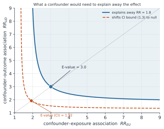
An unmeasured confounder $U$ distorts an estimate through two associations: how strongly it is linked to the exposure ( $RR_{EU}$ ) and how strongly to the outcome ( $RR_{UD}$ ), each expressed as a risk ratio. VanderWeele & Ding (2017) showed the maximum factor by which such a confounder can inflate an observed risk ratio is

$B = \frac{RR_{EU}\,RR_{UD}}{RR_{EU} + RR_{UD} - 1},$

with no assumptions about the confounder’s distribution or direction. Setting $B$ equal to the observed $RR$ traces the curve of confounder strengths that would just explain the effect away (Figure 1); anything above the curve more than explains it.

The E-value#

The E-value is the single number on that curve where the two required associations are equal — the minimum strength, on both the exposure and outcome sides, that an unmeasured confounder would need to reduce the observed association to the null:

$\text{E-value} = RR + \sqrt{RR\,(RR - 1)},$

for an observed risk ratio $RR \ge 1$ (use $1/RR$ if it is protective). Report it for the point estimate and, separately, for the confidence-interval limit closest to the null — the latter asks how much confounding would make the result statistically null, a stricter bar. An E-value is not a probability that confounding exists; it is a yardstick for the conversation about robustness, to be judged against how strong measured confounders actually are.

Bigger effects are harder to explain away#

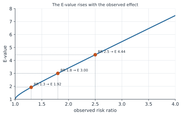
The E-value rises with the observed effect: a barely-elevated risk ratio evaporates under mild confounding, while a large one demands an implausibly strong hidden common cause (Figure 2). That is the intuition behind the old dictum that strong associations are harder to confound — the E-value just makes it quantitative.

Figure 2. The E-value rises with the observed risk ratio: RR 1.3 has an E-value of 1.92, RR 1.8 gives 3.0, and RR 2.5 gives 4.4. Weak effects are fragile to confounding; strong ones are robust.

A worked example#

Suppose an adjusted analysis reports a risk ratio of $1.8$ (95% CI $1.3$ – $2.5$ ).

Python

import numpy as np

def evalue(rr):
    rr = rr if rr >= 1 else 1 / rr            # protective effects: use the reciprocal
    return rr + np.sqrt(rr * (rr - 1))

rr, ci_low = 1.8, 1.3
print(f"E-value (point estimate) {evalue(rr):.2f}")
print(f"E-value (CI limit)       {evalue(ci_low):.2f}")

E-value (point estimate) 3.00
E-value (CI limit)       1.92

The point-estimate E-value is $3.0$ : an unmeasured confounder would need to be associated with both the exposure and the outcome by a risk ratio of at least $3$ — and be unaccounted for by every measured covariate — to explain away the finding. The CI-limit E-value of $1.92$ says confounding on the order of a risk ratio of $1.9$ would already render the result statistically null. Whether those are plausible is a subject-matter judgment: compare them to the strongest measured confounder in the study.

The E-value is the most transportable summary, but not the only sensitivity tool:

Rosenbaum bounds — for matched studies, the factor $\Gamma$ by which two matched units’ odds of treatment could differ due to hidden bias before the conclusion changes.
Tipping-point / bias-function analysis — posit a confounder with specified associations and re-estimate, finding where the effect crosses the null.
Negative controls — an exposure or outcome that should show no effect; a non-null result there flags residual confounding.

Why it matters#

Observational studies dominate epidemiology precisely where randomization is impossible, and their central vulnerability is always the confounder nobody measured. An estimate reported without any sensitivity analysis quietly asks the reader to assume that vulnerability away; an E-value replaces that silence with a number, turning “there could be confounding” into “confounding this strong, on both arms, unexplained by everything measured — is that plausible here?” It is the natural last step after any of the adjustment methods on this site: those make the measured confounders comparable, and the E-value states, in one figure, how much the unmeasured ones could still matter.