Hardy–Weinberg Equilibrium

Hardy–Weinberg equilibrium (HWE) is the null model of population genetics: it says how genotype frequencies relate to allele frequencies when nothing interesting is happening. Deviations from it are how we detect inbreeding, natural selection, hidden population structure, and — very practically — genotyping errors in a sequencing pipeline.

Left: the Hardy–Weinberg genotype frequencies are the terms of — , , — with the heterozygote frequency peaking at when . Right: starting from three arbitrary genotype distributions, the heterozygote frequency snaps to its Hardy–Weinberg value after a single generation of random mating and stays there, regardless of the starting point. — Figure 1. Left: the Hardy–Weinberg genotype frequencies are the terms of $(p+q)^2$ — $p^2$ , $2pq$ , $q^2$ — with the heterozygote frequency $2pq$ peaking at $0.5$ when $p=0.5$ . Right: starting from three arbitrary genotype distributions, the heterozygote frequency snaps to its Hardy–Weinberg value $2pq$ after a single generation of random mating and stays there, regardless of the starting point.

The equilibrium#

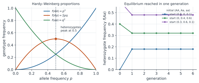
Consider a single biallelic locus with alleles $A$ and $a$ . Let $p$ be the frequency of allele $A$ and $q = 1 - p$ the frequency of allele $a$ . Under random mating, an individual’s two alleles are like two independent draws from the allele pool, so the genotype frequencies are the terms of $(p+q)^2$ : $f(AA) = p^2, \qquad f(Aa) = 2pq, \qquad f(aa) = q^2.$ These are the Hardy–Weinberg proportions, and they are reached after a single generation of random mating regardless of the starting genotype frequencies (Figure 1).

Show that one generation of random mating reaches equilibrium

Start from arbitrary genotype frequencies $f_{AA}, f_{Aa}, f_{aa}$ — not necessarily in Hardy–Weinberg proportions. The allele frequency in the gamete pool is

$p = f_{AA} + \tfrac12 f_{Aa}, \qquad q = f_{aa} + \tfrac12 f_{Aa} = 1 - p .$

Random mating is the random union of two gametes, so an offspring’s two alleles are independent draws from this pool:

$f'_{AA} = p^2, \qquad f'_{Aa} = 2pq, \qquad f'_{aa} = q^2 .$

These are the Hardy–Weinberg proportions, reached in a single generation. They are also a fixed point: the new allele frequency is $p' = f'_{AA} + \tfrac12 f'_{Aa} = p^2 + pq = p(p+q) = p$ , so the frequencies stay put every generation thereafter.

Once reached, both the allele frequencies and the genotype frequencies stay constant generation after generation — hence “equilibrium”.

Assumptions#

The result holds when the idealizing assumptions of the model are met.

Random mating (no assortative mating or inbreeding).
No selection: all genotypes have equal survival and fertility.
No mutation changing one allele into another.
No migration (gene flow) from populations with different allele frequencies.
A large population, so that genetic drift does not perturb the frequencies by chance sampling.

Because the model treats an individual as two independent allele draws, the genotype probability $2pq$ for heterozygotes carries the factor $2$ : the ordered outcomes $Aa$ and $aA$ are both heterozygous.

Testing for HWE#

Given observed genotype counts in a sample of $N$ individuals, we can test whether the population is consistent with HWE.

Estimating the allele frequency#

Each individual carries two alleles, so with observed counts $n_{AA}$ , $n_{Aa}$ , $n_{aa}$ (summing to $N$ ) the allele-frequency estimate is $\hat p = \frac{2 n_{AA} + n_{Aa}}{2N}, \qquad \hat q = 1 - \hat p .$

The chi-square goodness-of-fit test#

Under the null hypothesis of HWE, the expected counts are $E_{AA} = \hat p^2 N$ , $E_{Aa} = 2\hat p\hat q N$ , and $E_{aa} = \hat q^2 N$ . The Pearson chi-square statistic compares observed and expected counts: $\chi^2 = \sum_{g \in \{AA,Aa,aa\}} \frac{(O_g - E_g)^2}{E_g}.$ There are three genotype categories, but we lose one degree of freedom for the total count constraint and one more for estimating $\hat p$ from the data, leaving $3 - 1 - 1 = 1$ degree of freedom for a biallelic locus. A large statistic (small p-value relative to the $\chi^2_1$ distribution) is evidence against HWE.

Worked example#

Suppose we genotype $N = 200$ individuals and observe $n_{AA} = 90$ , $n_{Aa} = 60$ , $n_{aa} = 50$ .

First estimate the allele frequency: $\hat p = \frac{2(90) + 60}{2(200)} = \frac{240}{400} = 0.6, \qquad \hat q = 0.4 .$ Then the expected counts under HWE are $E_{AA} = 0.6^2 \cdot 200 = 72, \quad E_{Aa} = 2(0.6)(0.4)\cdot 200 = 96, \quad E_{aa} = 0.4^2 \cdot 200 = 32 .$ The chi-square statistic is $\chi^2 = \frac{(90-72)^2}{72} + \frac{(60-96)^2}{96} + \frac{(50-32)^2}{32} = 4.5 + 13.5 + 10.125 = 28.125 .$ Against $\chi^2_1$ , the $5\%$ critical value is $3.84$ , so $28.125$ is highly significant ( $p \approx 10^{-7}$ ). The sample has far too few heterozygotes and too many homozygotes — the classic signature of a heterozygote deficit.

What deviations mean#

A significant departure from HWE is a signal, not a diagnosis, and the direction is informative.

Heterozygote deficit (as above) commonly indicates inbreeding, a Wahlund effect from pooling structured subpopulations (see population structure), or genotyping error such as allele dropout.
Heterozygote excess can indicate outbreeding, overdominant selection, or contamination.
In genome-wide data, HWE filtering is a routine quality-control step: markers that fail HWE badly in controls usually reflect assay artefacts and are removed before running a GWAS.

In code#

R#

obs <- c(AA = 90, Aa = 60, aa = 50)
N <- sum(obs)
phat <- (2 * obs["AA"] + obs["Aa"]) / (2 * N)   # 0.6
qhat <- 1 - phat
exp_freq <- c(AA = phat^2, Aa = 2 * phat * qhat, aa = qhat^2)
expected <- exp_freq * N                          # 72, 96, 32

chisq <- sum((obs - expected)^2 / expected)       # 28.125
pval  <- pchisq(chisq, df = 1, lower.tail = FALSE) # ~ 1.1e-07
c(chisq = chisq, pval = pval)

# chisq.test uses df = 2 by default (does not know p was estimated),
# so compute the 1-df p-value manually as above.

Python#

Python

import numpy as np
from scipy import stats

obs = np.array([90, 60, 50])          # AA, Aa, aa
N = obs.sum()
phat = (2 * obs[0] + obs[1]) / (2 * N)  # 0.6
qhat = 1 - phat
expected = np.array([phat**2, 2 * phat * qhat, qhat**2]) * N  # [72, 96, 32]

chisq = np.sum((obs - expected)**2 / expected)   # 28.125
pval = stats.chi2.sf(chisq, df=1)                # ~ 1.1e-07
print(chisq, pval)

28.124999999999993 1.1372725656979712e-07

Julia#

Julia

using Distributions

obs = [90, 60, 50]                # AA, Aa, aa
N = sum(obs)
phat = (2obs[1] + obs[2]) / (2N)  # 0.6
qhat = 1 - phat
expected = [phat^2, 2phat*qhat, qhat^2] .* N   # [72.0, 96.0, 32.0]

chisq = sum((obs .- expected).^2 ./ expected)  # 28.125
pval = ccdf(Chisq(1), chisq)                   # ~ 1.1e-7
println((chisq, pval))

Why it matters#

Hardy–Weinberg equilibrium is the reference point against which almost every population-genetic observation is measured. Because it converts allele frequencies into expected genotype frequencies under a clean set of assumptions, any deviation localizes an interesting force — mating structure, selection, or subdivision — and its routine use as a quality-control filter keeps spurious markers out of downstream association analyses.