p-Values

The p-value is among the most reported—and most misunderstood measures in epidemiology. It quantifies how surprising the data are under the null hypothesis, and understanding exactly what it does and does not say is essential for honest inference. Furthermore, the p-value can be taken as a continuous measure of the plausibility of the null hypothesis given the data.

Left: the two-sided p-value for the worked example is the standard-normal tail mass beyond , totalling about . Right: when is true the p-value is Uniform — a histogram of 10,000 simulated null p-values is flat, and the shaded region holds about of them, which is exactly why testing at gives a Type I error rate of . — Figure 1. Left: the two-sided p-value for the worked example is the standard-normal tail mass beyond $\pm 2.1$ , totalling about $0.0357$ . Right: when $H_0$ is true the p-value is Uniform $(0,1)$ — a histogram of 10,000 simulated null p-values is flat, and the shaded $p \le 0.05$ region holds about $5\%$ of them, which is exactly why testing at $\alpha$ gives a Type I error rate of $\alpha$ .

Definition#

The p-value is the probability, computed assuming the null hypothesis $H_0$ is true, of obtaining a test statistic at least as extreme as the one actually observed:

$p = \Pr(\,T \text{ at least as extreme as } t_{\text{obs}} \mid H_0\,).$

“At least as extreme” is determined by $H_a$ : one tail for a directional alternative, both tails for a two-sided one. Small p-values mean the data would be unusual if $H_0$ held, casting doubt on $H_0$ (i.e., the null hypothesis is less likely to be true).

What a p-value is NOT#

Small p-values are not everything.

It is not $\Pr(H_0 \text{ is true})$ (i.e., you cannot prove the alternative hypothesis only disprove the nyll). It conditions on $H_0$ ; it does not measure the probability of $H_0$ .
It is not the probability the result occurred “by chance.”
It is not the size or importance of an effect—a tiny, irrelevant effect can yield a small p-value with a large sample (it’s just a matter of the sample size).
$1-p$ is not the probability $H_a$ is true.

Relation to $\alpha$ #

The significance level $\alpha$ is a fixed threshold chosen before seeing data; we reject $H_0$ when $p \le \alpha$ . This keeps the Type I error rate (long run probability of rejecting the null given that the alternative is true) at $\alpha$ . The p-value itself is a continuous summary of evidence, not a yes/no verdict. Becuase of this, p-values should always be reported as continuous values, not just stars or crude buckets (e.g., “< 0.05”).

Worked example#

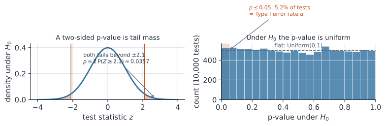
Suppose a standardized test statistic is $z_{\text{obs}} = 2.1$ under $H_0$ , with a standard normal reference and a two-sided alternative. The p-value is the mass in both tails beyond $2.1$ :

$p = 2\,\Pr(Z \ge 2.1) = 2 \times 0.0179 \approx 0.0357.$

Since $0.0357 < 0.05$ , we would reject $H_0$ at $\alpha=0.05$ . For a $t$ statistic we use the $t$ -distribution instead of the normal.

In code#

Compute p-values from a statistic using tail probabilities.

R#

z <- 2.1
2 * pnorm(z, lower.tail = FALSE)     # two-sided z p-value
t_stat <- 2.11; df <- 9
2 * pt(abs(t_stat), df, lower.tail = FALSE)   # two-sided t p-value

Python#

Python

from scipy import stats
z = 2.1
print(2 * stats.norm.sf(z))               # two-sided z
print(2 * stats.t.sf(abs(2.11), df=9))    # two-sided t

0.035728841125633085
0.06406977491571955

Julia#

Julia

using Distributions
z = 2.1
println(2 * ccdf(Normal(), z))                 # two-sided z
println(2 * ccdf(TDist(9), abs(2.11)))         # two-sided t

Simulation: under $H_0$ the p-value is Uniform(0,1)#

A key fact: if $H_0$ is true (and the test is exact), the p-value is uniformly distributed on $[0,1]$ (Figure 1). That is why rejecting when $p \le \alpha$ gives a Type I error rate of exactly $\alpha$ .

set.seed(7)
pvals <- replicate(10000, {
  x <- rnorm(30, mean = 0, sd = 1)     # H0: mean = 0 is TRUE
  t.test(x, mu = 0)$p.value
})
mean(pvals <= 0.05)   # ~0.05
hist(pvals)           # approximately flat

Why it matters for statistics#

The p-value is a calibrated measure of evidence against a null model, and its uniform-under- $H_0$ behavior is what makes significance testing control error rates. Interpreting it correctly—as conditional on $H_0$ , not a probability of $H_0$ —prevents the overclaiming that plagues applied research.