Hypothesis Testing

Hypothesis testing is the formal machinery epidemiologists use to decide whether an observed effect—a difference in infection rates, a shift in mean exposure—is more than noise. It frames a question as a decision between two competing claims about the world.

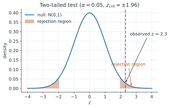
The null distribution with the two-tailed rejection region and an observed test statistic.

The two hypotheses

The null hypothesis $H_0$ states “no effect” or “no difference” (e.g., the mean equals a reference value).
The alternative hypothesis $H_a$ is what we entertain if the data are incompatible with $H_0$ (e.g., the mean differs).

We summarize the data with a test statistic—a single number whose distribution under $H_0$ is known.

The logic

The reasoning is a proof by contradiction under uncertainty: assume $H_0$ is true, then ask how surprising the observed data are. If data at least as extreme as ours would almost never occur when $H_0$ holds, we reject $H_0$ in favor of $H_a$ . The measure of surprise is the p-value.

Errors and significance level

Because we decide under uncertainty, two mistakes are possible:

	$H_0$ true	$H_0$ false
Reject $H_0$	Type I error (prob. $\alpha$ )	correct
Fail to reject	correct	Type II error (prob. $\beta$ )

The significance level $\alpha$ (often $0.05$ ) is the Type I error rate we are willing to tolerate; we reject $H_0$ when the p-value is below $\alpha$ . Power is $1-\beta$ .

Choosing a test by data type

Data	Question	Typical test
Continuous	mean vs. value / two means	z-test (known $\sigma$ ), $t$ -test
Proportions	success rate vs. value / two rates	binomial test, `prop.test`
Counts / categories	association in a table	chi-square, Fisher’s exact

Worked example: one-sample $t$ -test

Suppose we measure incubation times (days) for $n=10$ cases and want to test $H_0:\mu = 5$ against $H_a:\mu \ne 5$ . We observe $\bar{x}=5.8$ and $s=1.2$ . The test statistic is

$t = \frac{\bar{x}-\mu_0}{s/\sqrt{n}} = \frac{5.8 - 5}{1.2/\sqrt{10}} = \frac{0.8}{0.3795} \approx 2.11,$

compared to a $t$ -distribution with $n-1=9$ degrees of freedom. The two-sided p-value is about $0.064$ , so at $\alpha=0.05$ we would not reject $H_0$ .

In code

R

set.seed(42)
x <- rnorm(10, mean = 5.8, sd = 1.2)
t.test(x, mu = 5)                      # continuous: one-sample t-test
prop.test(x = 18, n = 40, p = 0.5)     # proportion vs. 0.5

Python

import numpy as np
from scipy import stats
rng = np.random.default_rng(42)
x = rng.normal(5.8, 1.2, size=10)
print(stats.ttest_1samp(x, popmean=5))          # continuous
print(stats.binomtest(18, 40, p=0.5))           # proportion

TtestResult(statistic=np.float64(1.1216087309978322), pvalue=np.float64(0.2910612434086062), df=np.int64(9))
BinomTestResult(k=18, n=40, alternative='two-sided', statistic=0.45, pvalue=0.6358280026288412)

Julia

using HypothesisTests, Random, Distributions
Random.seed!(42)
x = rand(Normal(5.8, 1.2), 10)
println(OneSampleTTest(x, 5.0))          # continuous
println(BinomialTest(18, 40, 0.5))       # proportion

Why it matters for statistics

Hypothesis testing gives a disciplined, reproducible rule for turning data into decisions while controlling the rate of false alarms. It is the foundation for evaluating treatment effects, screening associations, and reporting findings in nearly every quantitative study.