Model Interpretability and SHAP
A model that predicts a patient is high-risk is useless — or worse, dangerous — if no one can say why. Interpretability is what turns a black-box prediction into something a clinician can act on, a reviewer can audit, and a scientist can learn from, and in health settings it is often a requirement, not a luxury. This page surveys how to explain a model’s predictions, and then focuses on SHAP (SHapley Additive exPlanations), the method that has become the default because it rests on a uniqueness result from cooperative game theory: among all ways to divide a prediction among its features, only one is fair in a precise sense.
Why interpret a model#
Four distinct needs drive interpretability, and they ask for different things. Trust: a decision-maker will act on a prediction only if its reasoning is inspectable and sensible. Debugging: explanations expose when a model has learned a spurious shortcut — the dermatology classifier that keyed on a ruler beside malignant lesions was caught this way. Fairness: attributions reveal whether a model leans on a sensitive attribute, or a proxy for one, in ways that would be inequitable. Insight: sometimes the model has found a real pattern, and the explanation is the scientific finding. A useful split is global interpretability (how does the model behave overall — which features matter, in what direction) versus local (why this prediction for this case), and good tools provide both.
Model-agnostic explanations#
Several methods explain any model by probing it from the outside. Permutation importance measures a feature’s global importance by how much accuracy drops when its values are randomly shuffled, breaking its link to the outcome — model-agnostic and honest, unlike the impurity importance of tree ensembles. Partial-dependence and individual-conditional-expectation plots trace how the prediction changes as one feature is swept across its range, holding others fixed, showing the shape of a relationship. LIME explains a single prediction by fitting a simple, interpretable model to the black box’s behavior in a small neighborhood of that point. These are useful, but they can disagree and lack a principled account of how much each feature contributed — which is the gap SHAP fills.
SHAP and Shapley values#
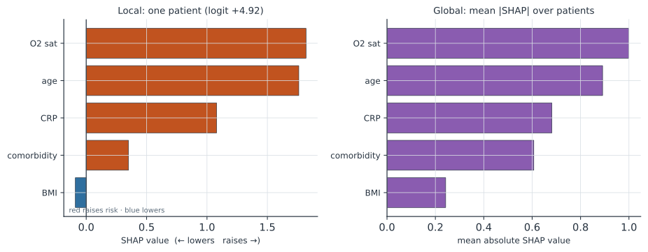
SHAP borrows the Shapley value, the game-theoretic answer to a fair-division problem: if features cooperate to produce a prediction, how much credit does each deserve? The Shapley value of feature averages its marginal contribution — how much the prediction changes when is added — over every possible order in which features could be added to the model: where is the set of features and is the model’s expected output knowing only the features in subset . This is the unique attribution satisfying four fairness axioms — efficiency (the contributions sum exactly to the prediction minus a baseline), symmetry, the dummy property, and additivity — which is what makes SHAP trustworthy where ad-hoc importances are not. The efficiency axiom is what the left of the figure shows: starting from the population base value (the average prediction), each feature’s pushes the output up or down, and they land exactly on this patient’s prediction. Averaging across many patients gives a principled global importance (right of the figure), so one method serves both scales. Exact Shapley values cost model evaluations, but TreeSHAP computes them exactly and fast for tree ensembles, and KernelSHAP approximates them for any model.
A worked example#
For a linear model , the Shapley values have a closed form: , the coefficient times the feature’s deviation from its mean. Suppose a logistic risk model has weight on standardized age, and a patient’s age is standard deviations above the mean (population mean ). That feature’s SHAP value is on the logit scale — a strong push toward risk — and the sum of all such pushes, added to the base logit, reproduces the model’s prediction exactly, the efficiency property in action.
In code#
Python#
SHAP values are exact and interpretable for a linear model, and permutation importance explains any model — both in a few lines:
import numpy as np
from sklearn.datasets import make_classification
from sklearn.linear_model import LogisticRegression
from sklearn.inspection import permutation_importance

X, y = make_classification(n_samples=1000, n_features=5, n_informative=3,
                           random_state=0)
clf = LogisticRegression().fit(X, y)
w, b, mean = clf.coef_[0], clf.intercept_[0], X.mean(0)

x = X[0]                                        # explain one patient
phi = w * (x - mean)                            # exact SHAP values (linear model)
base = b + w @ mean                             # baseline (average logit)
print("SHAP values:", np.round(phi, 2))
print(f"base {base:.2f} + sum(SHAP) {phi.sum():.2f} = {base + phi.sum():.2f}")
print(f"model logit (should match):            {w @ x + b:.2f}")

imp = permutation_importance(clf, X, y, n_repeats=20, random_state=0)
print("permutation importance:", np.round(imp.importances_mean, 3))
SHAP values: [ 0.54  0.05  0.32  0.52 -0.93]
base 0.02 + sum(SHAP) 0.50 = 0.52
model logit (should match):            0.52
permutation importance: [ 0.107 -0.003  0.007  0.011  0.061]
For nonlinear models the shap library computes the same attributions exactly and fast on a tree ensemble, and the efficiency property still holds — the base value plus the SHAP values reproduce the model’s output:
import shap, xgboost as xgb

model = xgb.XGBClassifier(n_estimators=150, max_depth=3, random_state=0).fit(X, y)
explainer = shap.TreeExplainer(model)
sv = explainer.shap_values(X)                        # exact SHAP, in log-odds units
print("global mean |SHAP| per feature:", np.round(np.abs(sv).mean(0), 2))

base = float(np.ravel(explainer.expected_value)[0])  # efficiency, on one patient
margin = float(model.predict(X[:1], output_margin=True)[0])
print(f"base {base:.2f} + sum(SHAP) {sv[0].sum():.2f} = {base + sv[0].sum():.2f}"
      f"  (model output {margin:.2f})")
global mean |SHAP| per feature: [1.79 1.68 1.52 1.14 1.5 ]
base -0.04 + sum(SHAP) 5.54 = 5.50  (model output 5.50)
In a notebook, shap.summary_plot(sv, X) draws the global beeswarm and shap.plots.waterfall(...) the per-patient explanation of the figure.
R#
# fastshap / treeshap for SHAP; iml and DALEX for model-agnostic explanations.
library(treeshap)
unified <- unify(xgb_model, X)              # convert the model
shaps <- treeshap(unified, X)$shaps         # per-row SHAP values
colMeans(abs(shaps))                        # global importance
Julia#
# ShapML.jl computes Shapley-based feature attributions for any model.
using ShapML, DataFrames
explain = DataFrame(X[1:5, :], :auto)
shap = ShapML.shap(explain = explain, model = model, predict_function = predict)
Why it matters#
In epidemiology and clinical prediction, an explanation is often what makes a model usable at all. SHAP turns a risk score into a per-patient statement — this patient is flagged mostly because of their oxygen saturation and age — that a clinician can sanity-check and a patient can be told, and its global view audits whether a surveillance or triage model is leaning on defensible signals rather than artefacts or protected attributes. Two cautions temper this. An explanation describes the model, not the world: a feature with a large SHAP value is influential in the model’s arithmetic, which is association, not a causal effect, and reading it as “reducing this feature would reduce risk” is a mistake. And explanations can be unstable or gamed, so they support human judgment rather than replacing it — the same posture every model on this site asks for.