Serocatalytic Models

A serosurvey measures who carries antibodies to a pathogen — the footprint of past infection. Plot that seroprevalence against age and it almost always rises: older people have had more years of exposure, so more of them have been infected at least once. The rate of that rise encodes the force of infection (FOI) — the per-capita rate at which susceptibles become infected — and a serocatalytic model is the machinery that reads the FOI back out of the age–seroprevalence curve. It is one of the few ways to estimate transmission intensity without ever observing a single transmission event.

The catalytic model#

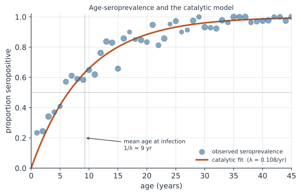
Treat infection as an irreversible transition from susceptible to seropositive, occurring at hazard $\lambda$ (the force of infection) — the same “catalytic” idea Muench borrowed from chemical kinetics. Under a constant FOI, the probability a person of age $a$ has been infected by now is the survival-analysis complement of never having been infected:

$P(\text{seropositive} \mid a) = 1 - e^{-\lambda a}.$

So seroprevalence approaches 1 exponentially with age, and the single parameter $\lambda$ sets the pace: the mean age at infection is $1/\lambda$ , and $\lambda$ connects directly to the basic reproduction number (roughly $R_0 \approx 1 + L/A$ for life expectancy $L$ and mean age at infection $A$ ). Fitting is a one-line generalized linear model — binomial seropositivity with a complementary-log-log link and $\log(\text{age})$ as an offset makes the intercept $\log\lambda$ .

The FOI shapes the curve#

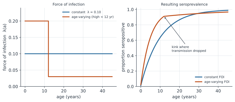
The constant-FOI model is only the start; the shape of the seroprevalence curve reveals how the FOI varies (Figure 2). A force of infection concentrated in childhood makes seroprevalence shoot up early and then flatten, leaving a kink at the age where transmission fell — the signature of a control programme, a past epidemic, or age-structured contact. So the model generalizes in two directions:

Age-varying FOI $\lambda(a)$ — piecewise-constant across age bands, giving $P(a) = 1 - \exp\!\big(-\!\int_0^a \lambda(u)\,du\big)$ ; a fitted peak flags the high-transmission ages.
Time-varying FOI $\lambda(t)$ — because a person’s seropositivity reflects the cumulative hazard over their lifetime, a cross-sectional serosurvey encodes transmission history, and the age pattern can be inverted to recover how the FOI changed over past calendar years.

Figure 2. A constant force of infection gives a smooth exponential rise; a force of infection concentrated in childhood makes seroprevalence climb steeply then flatten, leaving a kink where transmission dropped. Serosurveys are read backward through this mapping.

Real antibodies also wane, so the reversible catalytic model adds a seroreversion rate $\rho$ : seroprevalence then plateaus below 1 at $\lambda/(\lambda+\rho)$ rather than approaching it, and ignoring waning biases the FOI.

A worked example#

An age-stratified serosurvey of 45 age groups, generated under a constant FOI of $0.1$ /year.

Python

import numpy as np
import statsmodels.api as sm

rng = np.random.default_rng(9)
ages = np.arange(1, 46)
n = rng.integers(20, 45, len(ages))                 # sampled per age
pos = rng.binomial(n, 1 - np.exp(-0.10 * ages))     # seropositive counts

# catalytic model as a binomial GLM: cloglog link, log(age) offset
#   cloglog(p) = log(-log(1 - p)) = log(lambda) + log(age)
fit = sm.GLM(np.column_stack([pos, n - pos]), np.ones((len(ages), 1)),
             family=sm.families.Binomial(sm.families.links.CLogLog()),
             offset=np.log(ages)).fit()
lam = np.exp(fit.params[0])
lo, hi = np.exp(fit.conf_int()[0])
print(f"force of infection  {lam:.3f}/yr  (95% CI {lo:.3f}-{hi:.3f})")
print(f"mean age at infection  {1 / lam:.1f} yr")

force of infection  0.108/yr  (95% CI 0.100-0.116)
mean age at infection  9.3 yr

The fit recovers a force of infection near $0.1$ per year and a mean age at infection around ten — meaning, in this population, a susceptible person faces about a $10\%$ annual chance of infection, and half are infected by their early school years.

In code#

R#

# binomial GLM with a complementary-log-log link and log(age) offset
fit <- glm(cbind(pos, n - pos) ~ 1, family = binomial(link = "cloglog"),
           offset = log(age), data = sero)
exp(coef(fit))            # the force of infection lambda
# the serosv / serofoi packages fit age- and time-varying FOI (incl. Bayesian)

Julia#

Julia

using GLM, DataFrames
fit = glm(@formula(seropos ~ 1), sero, Binomial(), CloglogLink(),
          offset = log.(sero.age))
exp(coef(fit)[1])         # lambda

Why it matters#

The force of infection is the quantity that turns a static serosurvey into a dynamic picture of transmission, and serocatalytic models are how endemic-disease epidemiology has estimated it for measles, malaria, dengue, hepatitis, and SARS-CoV-2 alike — often the only feasible route where case surveillance is incomplete. The age pattern of immunity tells you the mean age at infection (which shapes vaccination-age policy), whether transmission is falling (a downward kink), and where the remaining susceptibles are. Read carelessly — ignoring antibody waning, or assuming a constant FOI through an epidemic — it misleads; read well, it reconstructs a pathogen’s transmission history from a single cross-section of blood.