Split-Plot Designs

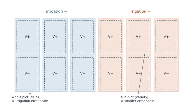
Some factors are simply harder to change than others. Irrigation is applied to a whole field; the crop variety can be planted row by row. A vaccine cold-chain temperature is set for an entire shipment; the assay run on each vial is chosen individually. A split-plot design embraces this: the hard-to-change factor is randomized to large whole plots, and the easy-to-change factor is randomized to sub-plots nested inside them — which means the two factors are compared with two different yardsticks of error.

Figure 1. A field split into whole plots that receive the hard-to-change factor (irrigation, shaded bands), each subdivided into sub-plots that receive the easy-to-change factor (variety, letters). The whole-plot factor is judged against variation between whole plots; the sub-plot factor and the interaction are judged against the smaller variation between sub-plots within a whole plot.

Two randomizations, two errors#

The defining feature is that randomization happens twice, at two scales:

The whole-plot factor (say irrigation, levels $\pm$ ) is assigned to whole plots. Its signal is compared against whole-plot error — the variation between whole plots treated alike.
The sub-plot factor (say variety) is assigned to sub-plots within each whole plot. It, and the whole-plot $\times$ sub-plot interaction, are compared against sub-plot error — the smaller variation between sub-plots inside a whole plot.

Because whole plots are few and large, whole-plot error has few degrees of freedom and is large; sub-plot error has many degrees of freedom and is small. The practical consequence is a precision trade-off: the sub-plot factor and the interaction are estimated more precisely than the whole-plot factor, even in the same experiment.

Warning

Analysing a split-plot as if it were a fully randomized two-factor design uses a single pooled error for everything. That tests the whole-plot factor against the wrong (too-small) denominator and badly overstates its significance — a classic error the design’s structure is meant to prevent.

The two-stratum ANOVA table#

For $a$ whole-plot levels replicated over $r$ whole plots each, with $b$ sub-plot levels, the ANOVA table separates into two blocks:

Source	df	Tested against
Whole-plot factor $A$	$a-1$	whole-plot error
Whole-plot error	$a(r-1)$	—
Sub-plot factor $B$	$b-1$	sub-plot error
Interaction $AB$	$(a-1)(b-1)$	sub-plot error
Sub-plot error	$a(r-1)(b-1)$	—

The horizontal rule between the two strata is the whole point: each factor sits above the error term that legitimately measures its replication.

A worked example#

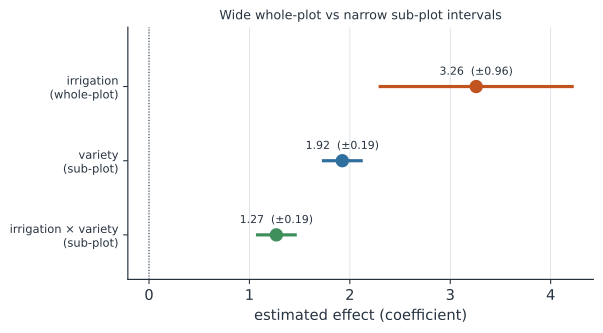
Two irrigation regimes ( $A_-$ , $A_+$ ) are each applied to three fields (whole plots); each field is split into two sub-plots planted with variety $B_-$ or $B_+$ . Irrigation has $a-1 = 1$ numerator df but only $a(r-1) = 4$ whole-plot-error df, so it is judged on the spread of just six fields. Variety and the irrigation $\times$ variety interaction each have $1$ df but are judged against $a(r-1)(b-1) = 4$ sub-plot-error df drawn from within-field contrasts, which are far less noisy. Fitting a mixed model with a random intercept per field recovers exactly this: the same-sized effect is reported with a wider interval for irrigation than for variety (Figure 2).

Figure 2. Estimated effects from the split-plot model with 95% intervals. The whole-plot (irrigation) effect carries a wide interval because it is measured against between-field variation; the sub-plot (variety) effect and the interaction carry narrow intervals because they are measured within fields.

In code#

R#

library(lme4)
# irrigation = whole-plot factor, variety = sub-plot factor, field = whole plot
fit <- lmer(yield ~ irrigation * variety + (1 | field), data = d)
# The random intercept (1 | field) is the whole-plot error stratum;
# the residual is the sub-plot error stratum. anova(fit) tests each factor
# against the appropriate denominator.
anova(fit)

Python#

Python

import numpy as np
import pandas as pd
import statsmodels.formula.api as smf

rng = np.random.default_rng(7)
rows = []
for irr in (-1, 1):
    for rep in range(3):                       # 3 fields per irrigation level
        field = f"{irr}_{rep}"
        u = rng.normal(0, 2.0)                 # whole-plot (field) effect
        for var in (-1, 1):
            y = 20 + 3 * irr + 2 * var + 1 * irr * var + u + rng.normal(0, 0.7)
            rows.append((field, irr, var, y))
d = pd.DataFrame(rows, columns=["field", "irrigation", "variety", "resp"])
m = smf.mixedlm("resp ~ irrigation * variety", d, groups=d["field"]).fit()
print(m.params[["irrigation", "variety", "irrigation:variety"]].round(2).to_dict())
print("SE:", m.bse[["irrigation", "variety"]].round(2).to_dict())

{'irrigation': 3.26, 'variety': 1.92, 'irrigation:variety': 1.27}
SE: {'irrigation': 0.49, 'variety': 0.1}

Julia#

Julia

using MixedModels, DataFrames
# (1 | field) captures the whole-plot error; the residual is sub-plot error
m = fit(MixedModel, @formula(yield ~ irrigation * variety + (1 | field)), d)

Why it matters for statistics#

Split-plot structure appears far more often than it is named — any time a treatment is applied to a group while another is applied within it, the data are split-plot whether or not the analyst notices. Field trials, multi-site clinical studies, repeated laboratory runs, and industrial experiments with a hard-to-reset machine setting all share this two-stratum error. Getting the ANOVA denominators right is not a technicality: it decides whether the headline (whole-plot) factor is being tested honestly or with a spuriously tiny error term.