Repeated Measures Designs

When you measure the same subjects under several conditions — or the same patients at several visits — the observations are not independent: a person who runs high on the first measurement tends to run high on the next. A repeated-measures design turns that correlation from a nuisance into an asset by using each subject as its own control, so the stable, person-to-person differences are swept out of the comparison. The payoff is power: within-subject contrasts can be dramatically tighter than the same comparison made between independent groups.

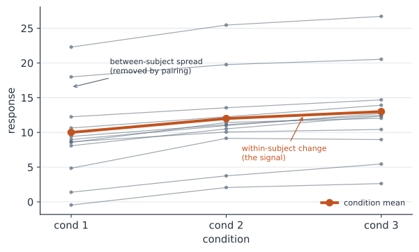
Figure 1. Individual subject trajectories across three conditions (thin lines) against the condition means (thick line). Subjects differ a lot in level — the lines are spread vertically — but each one moves in a similar way across conditions. A repeated-measures analysis compares the movement within each subject, removing the vertical spread that a between-subjects analysis would leave in the error term.

Within-subject versus between-subjects#

Split each observation $y_{ij}$ (subject $i$ , condition $j$ ) into a subject level and a condition effect:

$y_{ij} = \mu + s_i + \tau_j + \varepsilon_{ij}, \qquad s_i \sim \mathcal{N}(0, \sigma_s^2),\; \varepsilon_{ij} \sim \mathcal{N}(0, \sigma^2).$

A between-subjects comparison of two conditions lumps $\sigma_s^2$ (how much people differ) into the error, so the standard error is inflated by that person-to-person spread. A repeated-measures comparison differences the two measurements on the same subject, and $s_i$ cancels:

$y_{i2} - y_{i1} = (\tau_2 - \tau_1) + (\varepsilon_{i2} - \varepsilon_{i1}).$

The subject term is gone; only the within-subject noise $\sigma^2$ remains. Because measurements on one person are positively correlated, the variance of the difference is smaller than for two independent draws — the same reason a paired $t$ -test beats an unpaired one.

Compound symmetry and sphericity#

The simple model above implies compound symmetry: every pair of conditions has the same correlation. The ANOVA $F$ -test for repeated measures needs a slightly weaker condition, sphericity — that the variance of every pairwise difference $y_{ij} - y_{ij'}$ is the same. When it fails (common when conditions are time points, since nearby times correlate more than distant ones), the $F$ -test is too liberal and is corrected by shrinking its degrees of freedom (Greenhouse–Geisser, Huynh–Feldt), or the data are fit with a mixed model that models the correlation directly.

A worked example#

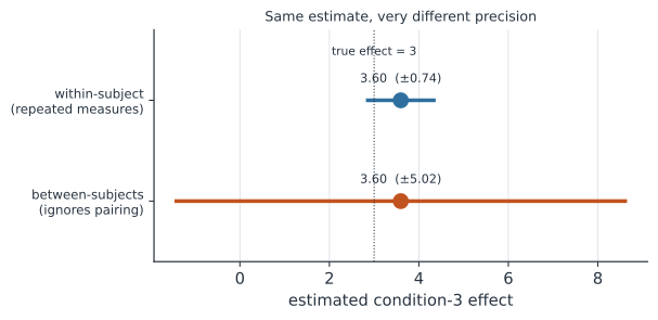
Twelve subjects are each measured under three conditions. People differ substantially in their baseline level ( $\sigma_s = 4$ ), but the within-subject noise is small ( $\sigma = 1$ ). A between-subjects analysis that ignored the pairing would carry the full baseline spread in its error bars; the repeated-measures analysis differences it away, so the condition effects come out with intervals several times narrower (Figure 2).

Figure 2. The condition effect estimated two ways from the same data. The between-subjects analysis (wide interval) carries person-to-person variability in its error; the within-subject repeated-measures analysis (narrow interval) removes it, sharpening the same estimate.

In code#

R#

library(lme4)
# subject as a random intercept removes person-to-person level differences
fit <- lmer(y ~ condition + (1 | subject), data = d)
# Compare with a between-subjects fit that ignores the pairing:
between <- lm(y ~ condition, data = d)   # wider SEs — subject variance in error

Python#

Python

import numpy as np
import pandas as pd
import statsmodels.formula.api as smf

rng = np.random.default_rng(3)
n_subj = 12
subj_level = rng.normal(0, 4.0, n_subj)           # big between-subject spread
tau = {"c1": 0.0, "c2": 2.0, "c3": 3.0}           # condition effects
rows = []
for i in range(n_subj):
    for c, t in tau.items():
        rows.append((i, c, 10 + subj_level[i] + t + rng.normal(0, 1.0)))
d = pd.DataFrame(rows, columns=["subject", "condition", "y"])

within = smf.mixedlm("y ~ condition", d, groups=d["subject"]).fit()
between = smf.ols("y ~ condition", d).fit()
print("within  SE(c3):", round(within.bse["condition[T.c3]"], 2))
print("between SE(c3):", round(between.bse["condition[T.c3]"], 2))

within  SE(c3): 0.38
between SE(c3): 2.56

Julia#

Julia

using MixedModels, DataFrames
# (1 | subject) removes the subject-level differences from the error term
within = fit(MixedModel, @formula(y ~ condition + (1 | subject)), d)

Why it matters for statistics#

Repeated-measures designs are everywhere in longitudinal epidemiology and clinical research: cohort visits, pre/post interventions, serial biomarker measurements, animals followed over time. Treating the repeated observations as independent double-counts information and produces confidence intervals that are wrong in both directions — too narrow for between-subject effects, too wide for within-subject ones. Recognizing the subject as a blocking factor, and modelling the within-subject correlation, is what makes the analysis both honest and powerful; the crossover trial is the special case where the “conditions” are treatments given in sequence.