Stepped-Wedge Designs

A stepped-wedge trial rolls an intervention out to clusters — clinics, wards, villages — one group at a time, in a randomized order, until everyone has crossed over. It is the design of choice when the intervention is expected to do good (so withholding it from a control arm for the whole study is hard to justify) and when a staggered rollout is logistically necessary anyway. Every cluster contributes both control and intervention time, and crosses over exactly once, in the forward direction only.

Figure 1. The stepped-wedge grid: clusters as rows, time periods as columns, cells shaded once a cluster has switched from control to intervention. Randomization sets the order in which clusters step over; by the final period all are exposed. Because later periods are more intervened and also simply later, the intervention effect must be separated from any secular time trend.

Time is confounded with rollout#

The defining hazard is built into the shape. Early periods are mostly control and late periods are mostly intervention — but late periods are also just later, so any secular trend (a seasonal change, an improving standard of care, an unrelated outbreak waning) masquerades as an intervention effect. A naïve before-versus-after comparison is therefore biased; the analysis must include a term for calendar time. The standard model is a linear mixed model with a fixed effect for each time period, a fixed effect for intervention exposure, and a random intercept per cluster:

$y_{ijk} = \mu + \beta_j + \theta\, X_{ij} + c_i + \varepsilon_{ijk}, \qquad c_i \sim \mathcal{N}(0, \sigma_c^2),$

where $\beta_j$ is the effect of period $j$ , $X_{ij} \in \{0,1\}$ marks whether cluster $i$ is under the intervention at period $j$ , and $\theta$ is the treatment effect of interest. Identifying $\theta$ separately from the $\beta_j$ is possible only because different clusters switch at different times — the randomized order is what breaks the confounding.

Where the information comes from#

The treatment effect is estimated from two directions at once: within clusters (before versus after each one steps over) and between clusters (at a given period, those already switched versus those not yet). Both comparisons are adjusted for the period effects, so the design is efficient but leans heavily on the modelling assumptions — a mis-specified time trend leaks straight into $\hat\theta$ .

Note

The cluster random intercept $c_i$ matters as much here as in any hierarchical model: observations in the same cluster are correlated, and ignoring that (analysing individuals as independent) understates the standard error of $\hat\theta$ , sometimes drastically.

A worked example#

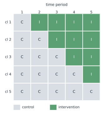
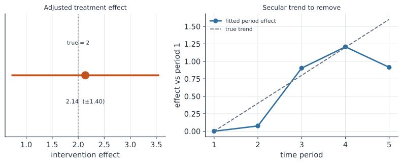
Four clusters are followed over five periods; one additional cluster crosses to the intervention at each period after a common baseline, so the exposure pattern forms the staircase in Figure 1. The truth is a treatment effect of $\theta = 2$ laid on top of a gently rising secular trend. A before/after contrast would over-count that trend, but the mixed model with period fixed effects recovers $\theta$ cleanly, and reports it alongside the estimated time trend it had to remove (Figure 2).

Figure 2. Left: the estimated intervention effect with its 95% interval, recovered after adjusting for calendar time. Right: the fitted period effects, the secular trend the design must separate from the rollout — the naive before/after estimate is inflated by exactly this trend.

In code#

R#

library(lme4)
# period as a fixed factor removes the secular trend; (1 | cluster) is the
# cluster random effect. treatment is the 0/1 exposure indicator X_ij.
fit <- lmer(y ~ treatment + factor(period) + (1 | cluster), data = d)

Python#

Python

import numpy as np
import pandas as pd
import statsmodels.formula.api as smf

rng = np.random.default_rng(5)
n_clusters, n_periods = 5, 5
switch = {c: c + 1 for c in range(n_clusters)}      # cluster c switches at period c+1
rows = []
for c in range(n_clusters):
    u = rng.normal(0, 1.5)                           # cluster random intercept
    for p in range(n_periods):
        X = int(p >= switch[c])                      # under intervention yet?
        y = 10 + 0.4 * p + 2.0 * X + u + rng.normal(0, 1.0)  # trend + effect
        rows.append((c, p, X, y))
d = pd.DataFrame(rows, columns=["cluster", "period", "treatment", "y"])
m = smf.mixedlm("y ~ treatment + C(period)", d, groups=d["cluster"]).fit()
print("treatment effect:", round(m.params["treatment"], 2),
      "SE:", round(m.bse["treatment"], 2))

treatment effect: 2.14 SE: 0.72

Julia#

Julia

using MixedModels, DataFrames
# period fixed effects absorb the secular trend; (1 | cluster) is the cluster RE
m = fit(MixedModel, @formula(y ~ treatment + period + (1 | cluster)), d)

Why it matters for statistics#

Stepped-wedge trials have become common in health-systems and implementation research — infection-control bundles, screening programmes, vaccination campaigns rolled out district by district — precisely where a parallel cluster-randomized trial is impractical or unethical. Their strength is that everyone eventually benefits and each cluster is partly its own control; their weakness is a hard dependence on correctly modelling calendar time and cluster correlation. The design is a vivid case of the section’s recurring theme: the ANOVA/mixed-model structure you fit has to mirror the structure by which the data were generated, or the headline effect is biased.