Crossover Designs
A crossover trial gives every subject every treatment, one after another, and compares the treatments within each person. Because the comparison is within-subject, the stable differences between people — the dominant source of variability in most biological measurements — cancel out, so a crossover can reach the same power as a parallel-group trial with far fewer participants. The price is a set of order effects you must design against: the treatment given first can leave a residue that colours the second period.
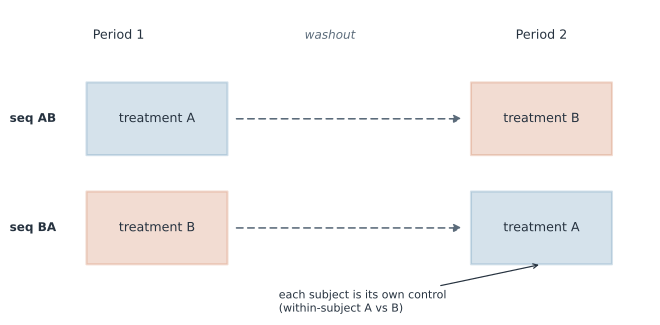
The 2×2 crossover#
In the simplest design, subjects are randomized to one of two sequences: AB (treatment A then B) or BA. Each subject is measured at the end of each period, with a washout in between long enough for the first treatment to clear. Three effects compete to explain the two measurements:
- the treatment effect (A versus B) — the quantity of interest;
- a period effect (period 2 differs from period 1 for everyone, e.g. disease progression or familiarity);
- a carryover effect (the previous treatment still acting in the next period).
Model the response for subject in period as
where is the treatment subject receives in period and is the subject’s level.
Separating treatment from period#
Differencing the two periods within a subject removes entirely — that is the whole point of the crossover. Comparing those within-subject differences between the two sequences then separates treatment from period, because the sequences see the same period effect but opposite treatment orders:
The period effect comes from the sum of the same within-subject differences.
In the 2×2 design, carryover is aliased with the sequence (between-subject) contrast, so it can only be estimated from the least precise comparison in the study — and testing for it then adjusting is unreliable. The robust fix is design, not analysis: make the washout long enough that . Higher-order designs (more periods or sequences, e.g. ABB/BAA) de-alias carryover and let it be estimated within subjects.
A worked example#
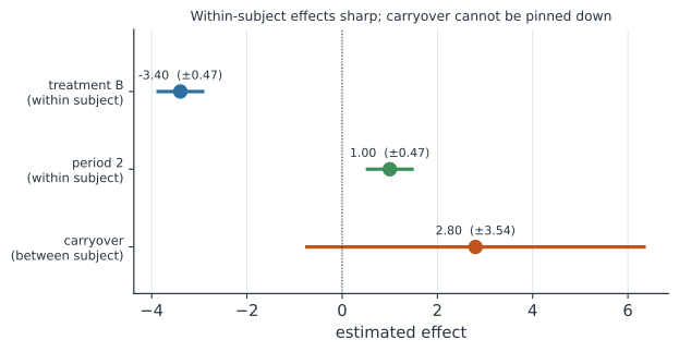
Twenty-four subjects are split between the AB and BA sequences; treatment B lowers the response by relative to A, and period 2 sits above period 1 for everyone. The between-subject spread () dwarfs the within-subject noise (). A within-subject analysis estimates the treatment and period effects with tight intervals, while the carryover contrast — forced through the between-subject comparison — comes out with an interval several times wider, showing exactly why the 2×2 design leans on washout rather than on estimating (Figure 2).
In code#
R#
library(lme4)
# treatment and period are within-subject; (1 | subject) removes subject level
fit <- lmer(y ~ treatment + period + (1 | subject), data = d)
# Classic hand analysis: within-subject period differences, compared by sequence
# tau_hat = 0.5 * (mean(d | AB) - mean(d | BA)),  d = y_period1 - y_period2
Python#
import numpy as np
import pandas as pd
import statsmodels.formula.api as smf

rng = np.random.default_rng(11)
seqs = {"AB": ("A", "B"), "BA": ("B", "A")}
eff = {"A": 0.0, "B": -3.0}                        # treatment B lowers response by 3
rows = []
sid = 0
for seq, (t1, t2) in seqs.items():
    for _ in range(12):                            # 12 subjects per sequence
        s = rng.normal(0, 5.0)                     # big subject level
        for period, t in [(1, t1), (2, t2)]:
            y = 20 + s + 1.0 * (period - 1) + eff[t] + rng.normal(0, 1.0)
            rows.append((sid, seq, period, t, y))
        sid += 1
d = pd.DataFrame(rows, columns=["subject", "seq", "period", "treatment", "y"])
m = smf.mixedlm("y ~ treatment + C(period)", d, groups=d["subject"]).fit()
print("treatment B:", round(m.params["treatment[T.B]"], 2),
      "period 2:", round(m.params["C(period)[T.2]"], 2))
treatment B: -3.4 period 2: 1.0
Julia#
using MixedModels, DataFrames
# within-subject treatment and period effects; subject as random intercept
m = fit(MixedModel, @formula(y ~ treatment + period + (1 | subject)), d)
Why it matters for statistics#
Crossover trials are a mainstay of studies on chronic, stable conditions — analgesics, antihypertensives, asthma controllers, bioequivalence — where each patient can serve as their own control and the treatment washes out between periods. They are a repeated-measures design with treatments as the repeated conditions, so they inherit both its power and its correlation structure, plus the special hazard of carryover. The lesson generalizes: when a design confounds an effect with your least precise contrast, the answer is usually to design that effect away rather than to trust a weak test of it.