Recurrent Networks and LSTMs

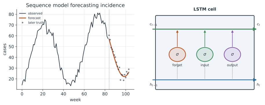
Case counts, wastewater signals, and syndromic-surveillance streams arrive as sequences: each week’s value depends on the weeks before it. A plain multilayer perceptron has no notion of order — shuffle its inputs and nothing changes — so it is the wrong tool for a time series. A recurrent neural network (RNN) fixes this by carrying a hidden state from one step to the next, a running summary of everything seen so far, and the long short-term memory (LSTM) cell refines the idea with gates that decide what to remember and what to forget.

Figure 1. Left: a recurrent model reads a weekly incidence series step by step and rolls its hidden state forward to forecast the coming weeks. Right: the LSTM cell, whose forget, input, and output gates protect a long-term cell state as it flows across many time steps.

The recurrent idea#

An RNN processes a sequence $\mathbf{x}_1, \mathbf{x}_2, \dots, \mathbf{x}_T$ one step at a time, updating a hidden state $\mathbf{h}_t$ that it carries forward: $\mathbf{h}_t = \phi\!\left(W_x \mathbf{x}_t + W_h \mathbf{h}_{t-1} + \mathbf{b}\right), \tag{1}$ where $W_x$ mixes in the current input, $W_h$ mixes in the previous hidden state, and $\phi$ is usually $\tanh$ . The prediction at each step is read off the hidden state, $\hat{y}_t = W_y \mathbf{h}_t + b_y$ . The same weights $W_x, W_h, W_y$ are reused at every step — the network is a single cell applied repeatedly, so it handles sequences of any length with a fixed number of parameters. Because $\mathbf{h}_t$ depends on $\mathbf{h}_{t-1}$ , which depends on $\mathbf{h}_{t-2}$ , and so on, (1) threads information from the distant past into the present prediction — the network has a memory.

Training uses backpropagation through time: unroll the recurrence into a deep feedforward network (one layer per time step, sharing weights), then apply ordinary backpropagation.

Why plain RNNs forget#

Unrolling over many steps is exactly where the simple RNN struggles. The gradient that carries the error from step $T$ back to step $t$ is a product of many Jacobian factors, one per intervening step. Multiply many numbers below one and the product vanishes; multiply many above one and it explodes. So a plain RNN’s gradient decays (or blows up) over long lags, and in practice it cannot learn dependencies more than a handful of steps apart — a fatal flaw when a seasonal disease signal links weeks that are a year apart.

The LSTM: a protected memory#

The LSTM solves the vanishing-gradient problem by adding a second state, the cell state $\mathbf{c}_t$ , that runs across the sequence along an almost-uninterrupted path — the horizontal conveyor belt at the top of the figure — regulated by three gates. Each gate is a sigmoid layer outputting values in $(0,1)$ that multiply a vector elementwise, acting as a soft switch. Writing $\sigma$ for the sigmoid and $\odot$ for the elementwise product, one LSTM step is $\begin{aligned} \mathbf{f}_t &= \sigma\!\left(W_f[\mathbf{h}_{t-1}, \mathbf{x}_t] + \mathbf{b}_f\right) &&\text{forget gate} \\ \mathbf{i}_t &= \sigma\!\left(W_i[\mathbf{h}_{t-1}, \mathbf{x}_t] + \mathbf{b}_i\right) &&\text{input gate} \\ \tilde{\mathbf{c}}_t &= \tanh\!\left(W_c[\mathbf{h}_{t-1}, \mathbf{x}_t] + \mathbf{b}_c\right) &&\text{candidate} \\ \mathbf{c}_t &= \mathbf{f}_t \odot \mathbf{c}_{t-1} + \mathbf{i}_t \odot \tilde{\mathbf{c}}_t &&\text{update cell state} \\ \mathbf{o}_t &= \sigma\!\left(W_o[\mathbf{h}_{t-1}, \mathbf{x}_t] + \mathbf{b}_o\right) &&\text{output gate} \\ \mathbf{h}_t &= \mathbf{o}_t \odot \tanh(\mathbf{c}_t) &&\text{hidden state.} \end{aligned}$ Read the cell-state update as the heart of it: the forget gate $\mathbf{f}_t$ chooses how much of the old memory $\mathbf{c}_{t-1}$ to keep, and the input gate $\mathbf{i}_t$ chooses how much of the new candidate $\tilde{\mathbf{c}}_t$ to write. When the forget gate stays near $1$ , the cell state passes through nearly unchanged and its gradient neither vanishes nor explodes — so the LSTM can carry a signal across hundreds of steps. The output gate $\mathbf{o}_t$ then decides how much of the memory to expose as this step’s hidden state and prediction. The gated recurrent unit (GRU) is a popular streamlined variant with two gates instead of three.

A worked example#

Suppose a scalar LSTM has learned to accumulate a seasonal level. At some step the previous cell state is $c_{t-1} = 2.0$ , the forget gate fires at $f_t = 0.9$ (keep most of the memory), the input gate at $i_t = 0.5$ , and the candidate is $\tilde{c}_t = 1.0$ . The new cell state is $c_t = 0.9 \times 2.0 + 0.5 \times 1.0 = 2.3$ : the memory is largely retained and nudged up. With an output gate $o_t = 0.8$ , the hidden state is $h_t = 0.8 \times \tanh(2.3) = 0.8 \times 0.980 = 0.784$ , which feeds the next step and the forecast. Notice that had the forget gate instead fired at $f_t = 0.1$ , almost all of the accumulated level would be discarded — the gates are how the network chooses its own memory horizon from the data.

In code#

Python#

The gate equations are the whole cell, so one forward pass is a few lines. Here a small LSTM cell (with fixed, illustrative weights) reads a short rising sequence and we watch its cell state accumulate — the mechanism, without training:

Python

import numpy as np
rng = np.random.default_rng(0)

def sigmoid(z):
    return 1 / (1 + np.exp(-z))

H = 4                                   # hidden/cell width
Wf, Wi, Wc, Wo = (0.3 * rng.standard_normal((H, H + 1)) for _ in range(4))
c = np.zeros(H); h = np.zeros(H)         # start with empty memory
sequence = [0.2, 0.5, 0.9, 1.4, 2.0]     # e.g. a rising weekly signal
for t, x in enumerate(sequence):
    z = np.concatenate([h, [x]])         # stack previous hidden state and input
    f = sigmoid(Wf @ z)                  # forget gate
    i = sigmoid(Wi @ z)                  # input gate
    c = f * c + i * np.tanh(Wc @ z)      # update the protected cell state
    o = sigmoid(Wo @ z)                  # output gate
    h = o * np.tanh(c)                   # expose part of the memory
    print(f"t={t}  x={x:.1f}  |c|={np.linalg.norm(c):.3f}  |h|={np.linalg.norm(h):.3f}")

t=0  x=0.2  |c|=0.060  |h|=0.030
t=1  x=0.5  |c|=0.177  |h|=0.090
t=2  x=0.9  |c|=0.342  |h|=0.181
t=3  x=1.4  |c|=0.537  |h|=0.303
t=4  x=2.0  |c|=0.750  |h|=0.454

For real forecasting you stack an LSTM layer under a linear read-out and train it by backpropagation through time; frameworks provide the cell and its gradients. A one-step-ahead case-count forecaster in PyTorch trains a real LSTM: window the past weeks, read the last hidden state, and predict the next week — here on a synthetic seasonal series, compared against a naive “next week equals this week” baseline.

Python

import torch, torch.nn as nn
torch.manual_seed(0)

wk = np.arange(160)                                  # standardized seasonal series
series = np.sin(2 * np.pi * wk / 52) + 0.3 * np.sin(2 * np.pi * wk / 13)
series = (series - series.mean()) / series.std()
look = 12                                            # 12 weeks -> next week
Xw = np.stack([series[i:i + look] for i in range(len(series) - look)])
yw = series[look:]
Xt = torch.tensor(Xw[:, :, None], dtype=torch.float32)   # (samples, steps, features)
yt = torch.tensor(yw[:, None], dtype=torch.float32)

class Forecaster(nn.Module):
    def __init__(self):
        super().__init__()
        self.lstm = nn.LSTM(1, 16, batch_first=True)
        self.head = nn.Linear(16, 1)
    def forward(self, x):
        out, _ = self.lstm(x)
        return self.head(out[:, -1])                 # read the last time step

net = Forecaster()
opt = torch.optim.Adam(net.parameters(), lr=0.01)
for epoch in range(300):
    opt.zero_grad()
    loss = nn.functional.mse_loss(net(Xt), yt)
    loss.backward(); opt.step()
naive = float(np.sqrt(np.mean((yw - Xw[:, -1]) ** 2)))   # persistence baseline
rmse = float(loss.item()) ** 0.5
print(f"LSTM train RMSE {rmse:.2f}  vs naive-persistence RMSE {naive:.2f}")
print(f"LSTM beats persistence: {rmse < naive}")

LSTM train RMSE 0.01  vs naive-persistence RMSE 0.19
LSTM beats persistence: True

For production forecasting you would split train/validation in time, tune the lookback and width, and — crucially — report calibrated prediction intervals, not just a point forecast.

R#

# torch for R provides nn_lstm; keras3 is the other common route.
library(torch)
net <- nn_module(
  initialize = function() {
    self$lstm <- nn_lstm(input_size = 1, hidden_size = 32, batch_first = TRUE)
    self$fc   <- nn_linear(32, 1)
  },
  forward = function(x) {
    out <- self$lstm(x)[[1]]
    self$fc(out[, dim(out)[2], ])        # read the last time step
  }
)

Julia#

Julia

# Flux's LSTM is a stateful recurrent layer you fold over a sequence.
using Flux
model = Chain(LSTM(1 => 32), Dense(32 => 1))
Flux.reset!(model)
forecast = [model([x]) for x in sequence]   # one output per step

Why it matters#

Recurrent networks are a data-driven counterpart to the mechanistic time-series tools elsewhere on this site. Where the renewal equation and compartmental models forecast incidence from an explicit transmission mechanism, an LSTM learns the temporal pattern directly from past case counts, wastewater, or search-trend series — useful for short-horizon nowcasting and forecasting when the mechanism is uncertain or the drivers are many. They shine when several noisy signals must be fused over time, and they are routinely combined with mechanistic models in ensemble forecasts. The usual cautions apply with force: a recurrent model extrapolates the patterns in its training data, so a genuinely novel dynamic — a new variant, a behavioural shift — is exactly what it has never seen, which is why calibrated uncertainty and mechanistic sanity checks belong alongside any neural forecast.