Graph Neural Networks

Much of the data that matters most in epidemiology is relational: who contacts whom, which places exchange travelers, how cases connect in a transmission tree, which regions border which. A neural network that treats each individual as an independent row throws that structure away. A graph neural network (GNN) keeps it, learning directly on the graph by letting each node exchange information with its neighbors — a scheme called message passing that generalizes the convolution of a CNN from a regular pixel grid to any graph at all.

Graphs in epidemiology#

A graph is a set of nodes joined by edges, and the field is full of them: contact and sexual-partnership networks, transmission networks and phylogenetic trees, mobility graphs linking cities by travel, spatial-adjacency graphs of counties (the structure behind areal disease-mapping models), and molecular graphs of drug and pathogen structures. Each node carries features — a person’s age and vaccination status, a county’s population and covariates — and often a label we want to predict, such as infection risk. The learning tasks come in three flavors: node classification (predict a label for each node, e.g. who is at risk), link prediction (predict missing or future edges, e.g. undocumented contacts or who infected whom), and graph classification (label a whole graph, e.g. flag an outbreak’s contact structure as super-spreading).

Message passing#

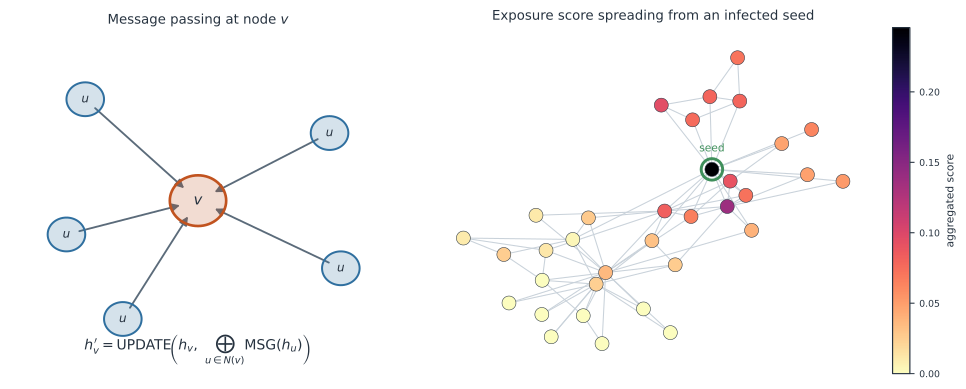
The core of every GNN is one operation, repeated: each node updates its hidden state by aggregating messages from its neighbors and combining them with its own state. Writing $h_v$ for node $v$’s embedding and $N(v)$ for its neighbors, one layer is $$h_v^{(k+1)} = \mathrm{UPDATE}\!\left(h_v^{(k)},\ \bigoplus_{u\in N(v)} \mathrm{MSG}\!\left(h_u^{(k)}\right)\right), \tag{1}$$ where $\mathrm{MSG}$ transforms each neighbor’s state (a learned linear map), $\bigoplus$ is a permutation-invariant aggregator — sum, mean, or max, so the result does not depend on how the neighbors are ordered — and $\mathrm{UPDATE}$ merges the aggregate with the node’s own state through a small network. Stacking $K$ such layers gives each node a receptive field of $K$ hops: after one layer a node knows its immediate contacts, after two it knows contacts-of-contacts, and so on — exactly the growing neighborhoods that matter for transmission. The right panel of the figure shows the aggregation alone, with no learning: starting from a single infected seed and repeatedly averaging over neighbors spreads an “exposure score” outward along the contact graph, the raw signal a trained GNN sharpens into a risk prediction.

The graph convolutional network#

The most common GNN layer, the graph convolutional network (GCN), makes the message-passing rule (1) concrete with a normalized neighbor-average followed by a linear map and a nonlinearity: $$H^{(k+1)} = \sigma\!\left(\hat A\, H^{(k)}\, W^{(k)}\right), \qquad \hat A = \tilde D^{-1/2}\tilde A\, \tilde D^{-1/2},$$ where $\tilde A = A + I$ is the adjacency matrix with self-loops added, $\tilde D$ is its diagonal degree matrix, $\hat A$ is the symmetric-normalized adjacency, $H^{(k)}$ stacks all node embeddings, and $W^{(k)}$ is the layer’s learned weights. The normalization by $\hat A$ keeps high-degree hubs from dominating the aggregate, and the whole layer is trained by backpropagation like any network. A CNN is the special case of this on a grid graph, which is why a GNN is often described as “convolution for irregular structure”; richer variants — GraphSAGE (sampling neighbors for scalability), graph attention networks (learning how much to weight each neighbor), and spatiotemporal GNNs (a GNN over the mobility graph feeding an LSTM over time) — all build on the same message-passing skeleton.

A worked example#

Take a tiny contact graph: node $A$ is connected to $B$ and $C$, and $B$ is also connected to $D$. Give each node a one-number feature — an infection indicator, $x = (1, 0, 0, 0)$ with only $A$ infected. One round of mean aggregation (including a self-loop) updates each node to the average of itself and its neighbors: $B$, touching the infected $A$, jumps from $0$ to about $0.33$; $C$ likewise; $D$, two hops from $A$, stays $0$ after one layer but rises after a second. That spreading average is (1) with a mean aggregator and identity message — the mechanism a GNN wraps in learned weights so that, instead of a fixed average, it learns what to pass and how to combine it to predict who becomes infected next.

In code#

Python#

The aggregation core of a GNN is a few lines of array math — here the normalized-adjacency propagation of an infection signal over a real contact network, the operation a GCN layer learns on top of:

import numpy as np
import networkx as nx

G = nx.karate_club_graph()                 # a 34-node social contact network
A = nx.to_numpy_array(G)
n = A.shape[0]
A_hat = A + np.eye(n)                       # add self-loops
deg = A_hat.sum(1)
S = A_hat / np.sqrt(deg)[:, None] / np.sqrt(deg)[None, :]   # normalized adjacency

x = np.zeros(n); x[0] = 1.0                 # one infected seed (node 0)
h = x.copy()
for _ in range(2):                          # two message-passing layers = 2-hop reach
    h = S @ h                               # aggregate neighbours' state
reached = int((h > 1e-9).sum())
top = np.argsort(h)[::-1][:4]
print(f"from 1 seed, {reached}/{n} nodes carry exposure signal after 2 hops")
print("highest-exposure nodes:", [(int(i), round(float(h[i]), 2)) for i in top])

from 1 seed, 26/34 nodes carry exposure signal after 2 hops
highest-exposure nodes: [(0, 0.25), (1, 0.14), (10, 0.09), (3, 0.09)]

A trained GCN wraps that aggregation in learned weights and a nonlinearity; with PyTorch Geometric a two-layer GCN classifies every node of the contact network above after seeing just two labelled examples — one per faction — by propagating their labels along the edges:

import torch, torch.nn as nn
from torch_geometric.nn import GCNConv
torch.manual_seed(0)

edges = np.array(list(G.edges())).T                  # the karate club from above
edge_index = torch.tensor(np.concatenate([edges, edges[::-1]], axis=1), dtype=torch.long)
labels = torch.tensor([0 if G.nodes[i]["club"] == "Mr. Hi" else 1 for i in G.nodes()])
feats = torch.eye(n)                                  # one-hot node identities

class GCN(nn.Module):                                 # 2 layers = 2-hop message passing
    def __init__(self):
        super().__init__()
        self.c1, self.c2 = GCNConv(n, 16), GCNConv(16, 2)
    def forward(self, x, ei):
        return self.c2(torch.relu(self.c1(x, ei)), ei)

gcn = GCN()
opt = torch.optim.Adam(gcn.parameters(), lr=0.02, weight_decay=5e-4)
seed = torch.zeros(n, dtype=torch.bool); seed[[0, 33]] = True   # 2 labelled nodes
for _ in range(120):                                  # semi-supervised training
    opt.zero_grad()
    loss = nn.functional.cross_entropy(gcn(feats, edge_index)[seed], labels[seed])
    loss.backward(); opt.step()
acc = (gcn(feats, edge_index).argmax(1) == labels).float().mean().item()
print(f"GCN labels all {n} nodes from 2 seeds: accuracy {acc:.2f}")

GCN labels all 34 nodes from 2 seeds: accuracy 0.97

R#

# Build the graph with igraph; train GNNs via the torch-for-R ecosystem.
library(igraph)
g   <- graph_from_adjacency_matrix(A, mode = "undirected")
Ahat <- A + diag(nrow(A))
d    <- rowSums(Ahat)
S    <- diag(1/sqrt(d)) %*% Ahat %*% diag(1/sqrt(d))   # normalized adjacency
h    <- as.vector(S %*% (S %*% x))                      # two message-passing layers

Julia#

# GraphNeuralNetworks.jl provides GNN layers on top of Flux.
using GraphNeuralNetworks, Flux
model = GNNChain(GCNConv(d_in => 32, relu), GCNConv(32 => 1))
ŷ = model(g, node_features)      # g is a GNNGraph of the contact network

Why it matters#

Graph neural networks let epidemiology model the thing that actually drives transmission — the network of contacts and movements — rather than pretending individuals are independent. On a contact network a GNN can predict who is most at risk from the pattern of their connections; on a mobility graph a spatiotemporal GNN can forecast where cases will travel next; on transmission data link prediction can reconstruct who infected whom; and on molecular graphs the same machinery predicts antimicrobial resistance or drug activity. The cautions are the network’s own: the graph must be measured (contact data are notoriously incomplete and biased), the model can leak or expose sensitive relationships, and — as with every model here — a GNN interpolates the structure it was trained on and must be validated out of sample before its predictions guide an intervention. Where the network science pages describe the structure of transmission, GNNs are how you learn on it.

Related#

• Networks and Graphs
• Centrality and Node Importance
• Networks in Ecology and Epidemiology
• Random-Graph Models
• Neural Networks and the Multilayer Perceptron
• Convolutional Networks and Image Identification
• Overfitting, Regularization, and Cross-Validation
• Quantitative Methods