Meta-Analysis

No single study is the last word. Meta-analysis is the machinery for combining estimates from many studies into one pooled estimate — sharper than any component, and honest about how much the studies disagree. It is the quantitative core of a systematic review, and it is really just a hierarchical model: each study measures its own true effect with error, and those true effects are themselves drawn from a distribution we want to characterize.

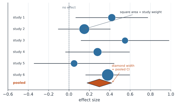
Fixed effect vs random effects#

Suppose study $i$ reports an estimate $y_i$ (a log odds ratio, a log risk ratio, a standardized mean difference) with within-study variance $v_i$ (so its standard error is $\sqrt{v_i}$). Both pooling models are inverse-variance weighted averages — precise studies count more — but they differ in what they assume the studies share.

A fixed-effect model assumes every study estimates the same effect $\theta$, and all disagreement is sampling error:

$$\hat\theta_{\text{FE}} = \frac{\sum_i w_i\, y_i}{\sum_i w_i}, \qquad w_i = \frac{1}{v_i}. \tag{1}$$

A random-effects model assumes each study has its own true effect $\theta_i \sim \mathcal{N}(\mu, \tau^2)$, and we want the mean $\mu$ of that distribution. It uses the same formula (1) but inflates every variance by the between-study variance $\tau^2$:

$$w_i^\* = \frac{1}{v_i + \tau^2}.$$

When $\tau^2 = 0$ the two coincide; when studies are heterogeneous, the random-effects model down-weights the large studies (they no longer dominate) and widens the pooled interval.

Heterogeneity: Q, τ², and I²#

How much do the true effects actually vary? Cochran’s Q compares observed dispersion to what sampling error alone predicts:

$$Q = \sum_i w_i (y_i - \hat\theta_{\text{FE}})^2,$$

which has expectation $k-1$ under homogeneity ($k$ studies). The DerSimonian–Laird estimate of the between-study variance is $\hat\tau^2 = \max\!\big(0,\ (Q - (k-1))/C\big)$ with $C = \sum w_i - \sum w_i^2 / \sum w_i$, and the widely-reported I² is the fraction of total variation that is between-study rather than sampling noise:

$$I^2 = \frac{Q - (k-1)}{Q} \times 100\%.$$

A worked example: pooling effect sizes#

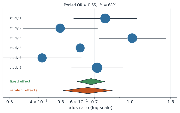
Six trials report a log odds ratio for the same intervention. The frequentist pooling, heterogeneity statistics, and prediction interval are a few lines of NumPy (Figure 2).

import numpy as np
from scipy import stats

# six studies: log odds ratio and its standard error
y = np.array([-0.25, -0.70, 0.02, -0.50, -0.88, -0.33])
se = np.array([0.16, 0.19, 0.17, 0.21, 0.20, 0.13])
k = len(y)
v = se**2
w = 1 / v

theta_fe = (w * y).sum() / w.sum()                      # fixed-effect pool
Q = (w * (y - theta_fe) ** 2).sum()
C = w.sum() - (w**2).sum() / w.sum()
tau2 = max(0.0, (Q - (k - 1)) / C)                      # DerSimonian-Laird
ws = 1 / (v + tau2)
theta_re = (ws * y).sum() / ws.sum()                    # random-effects pool
se_re = np.sqrt(1 / ws.sum())
I2 = max(0.0, (Q - (k - 1)) / Q) * 100
tcrit = stats.t.ppf(0.975, k - 2)
pi = theta_re + np.array([-1, 1]) * tcrit * np.sqrt(tau2 + se_re**2)

print(f"random-effects OR {np.exp(theta_re):.2f} "
      f"[{np.exp(theta_re-1.96*se_re):.2f}, {np.exp(theta_re+1.96*se_re):.2f}]")
print(f"Q={Q:.1f}  tau2={tau2:.3f}  I2={I2:.0f}%")
print(f"95% prediction interval for the OR: "
      f"[{np.exp(pi[0]):.2f}, {np.exp(pi[1]):.2f}]")

random-effects OR 0.65 [0.51, 0.84]
Q=15.7  tau2=0.063  I2=68%
95% prediction interval for the OR: [0.30, 1.43]

The pooled odds ratio is protective, but the prediction interval is wide enough to cross 1 — in a genuinely new setting the intervention might not help at all. That is exactly the caution $I^2$ alone would hide.

Bayesian meta-analysis and a Bayesian I²#

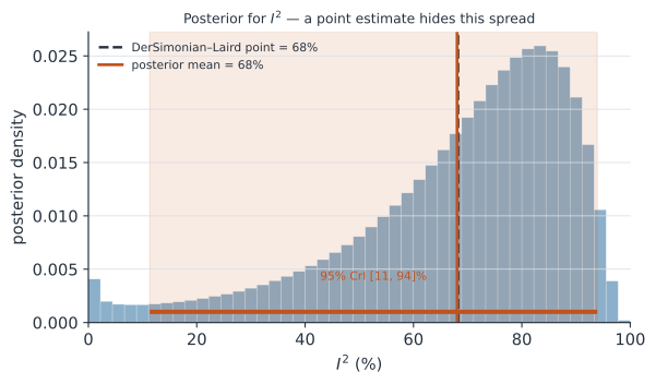
The random-effects model is a hierarchical model, so it is natural to fit it in a probabilistic programming language and get the full posterior — including the posterior of $\tau^2$, and hence of $I^2$. With only six studies the between-study variance is barely identified, so a weakly informative half-normal prior on $\tau$ is important (Röver et al. 2021). We compute $I^2$ at every posterior draw using Higgins & Thompson’s “typical” within-study variance $s^2$, turning a single number into a posterior distribution (Figure 3).

import jax.numpy as jnp
from jax import random
import numpyro
import numpyro.distributions as dist
from numpyro.infer import MCMC, NUTS

def meta(y, se):
    mu = numpyro.sample("mu", dist.Normal(0, 1))
    tau = numpyro.sample("tau", dist.HalfNormal(0.5))       # weakly informative
    with numpyro.plate("studies", len(y)):
        theta = numpyro.sample("theta", dist.Normal(mu, tau))
        numpyro.sample("obs", dist.Normal(theta, se), obs=y)

mcmc = MCMC(NUTS(meta), num_warmup=1000, num_samples=4000,
            num_chains=1, progress_bar=False)
mcmc.run(random.PRNGKey(0), y=jnp.array(y), se=jnp.array(se))
post = mcmc.get_samples()
mu_s, tau_s = np.array(post["mu"]), np.array(post["tau"])

s2 = (k - 1) * w.sum() / (w.sum() ** 2 - (w**2).sum())      # typical within-study var
I2_draws = tau_s**2 / (tau_s**2 + s2) * 100                 # Bayesian I^2, per draw
print(f"posterior OR {np.exp(mu_s.mean()):.2f} "
      f"[{np.exp(np.percentile(mu_s,2.5)):.2f}, {np.exp(np.percentile(mu_s,97.5)):.2f}]")
print(f"Bayesian I2 mean {I2_draws.mean():.0f}%  "
      f"95% CrI [{np.percentile(I2_draws,2.5):.0f}, {np.percentile(I2_draws,97.5):.0f}]%")

posterior OR 0.66 [0.49, 0.90]
Bayesian I2 mean 68%  95% CrI [12, 94]%

The posterior mean of $I^2$ lands close to the DerSimonian–Laird point estimate, but now comes with a wide credible interval — the honest statement is “substantial but poorly-determined heterogeneity,” not a single reassuring number.

Pooling disease prevalence#

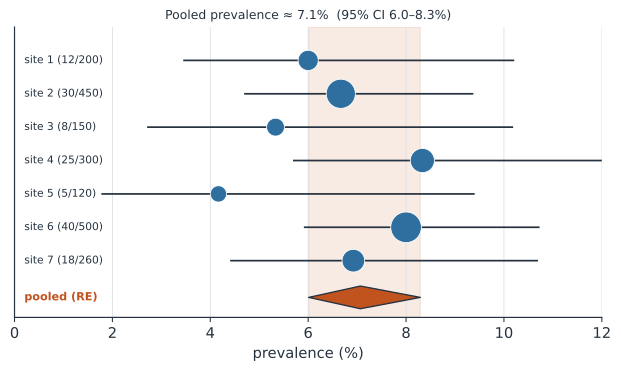
Meta-analysis also pools proportions — seroprevalence across sites, carriage rates across surveys. Prevalences are bounded in $[0,1]$ and their variance depends on the mean, so pooling raw proportions is a mistake. The classic two-step fix transforms first; the Freeman–Tukey double-arcsine transform was long the default, but it has a broken back-transformation and is now discouraged (Schwarzer et al. 2019; Röver & Friede 2022). The modern recommendation is a one-step binomial model on the logit scale (Lin & Chu 2020) — which is exactly a Bayesian random-effects logistic model, and keeps the pooled interval inside $[0,1]$ (Figure 4).

# seven sites: number positive out of number tested
pos = np.array([12, 30, 8, 25, 5, 40, 18])
ntot = np.array([200, 450, 150, 300, 120, 500, 260])

def prev_meta(pos, ntot):
    mu = numpyro.sample("mu", dist.Normal(-2.5, 1.0))       # logit-scale mean
    tau = numpyro.sample("tau", dist.HalfNormal(1.0))
    with numpyro.plate("sites", len(ntot)):
        a = numpyro.sample("a", dist.Normal(mu, tau))       # site logit
        numpyro.sample("obs", dist.Binomial(total_count=ntot, logits=a), obs=pos)

m = MCMC(NUTS(prev_meta), num_warmup=1000, num_samples=4000,
         num_chains=1, progress_bar=False)
m.run(random.PRNGKey(1), pos=jnp.array(pos), ntot=jnp.array(ntot))
mu_p = np.array(m.get_samples()["mu"])
pooled = 1 / (1 + np.exp(-mu_p))                            # back to prevalence
print(f"pooled prevalence {pooled.mean()*100:.1f}% "
      f"[{np.percentile(pooled,2.5)*100:.1f}, {np.percentile(pooled,97.5)*100:.1f}]%")

pooled prevalence 6.8% [5.3, 8.3]%

The same model in Stan#

The Bayesian random-effects meta-analysis is a natural fit for Stan. Driven from Python with PyStan, the model below reproduces the NumPyro fit almost exactly (pooled OR ≈ 0.66, $\tau$ ≈ 0.31, $I^2$ ≈ 69%). It is marked # no-run because the site build compiles no Stan toolchain, but it runs as-is once pystan is installed (pip install pystan).

# no-run
import stan, numpy as np

stan_code = """
data {
  int<lower=0> N;             // number of studies
  vector[N] y;                // observed effect (log odds ratio)
  vector<lower=0>[N] se;      // within-study standard error
}
parameters {
  real mu;                    // pooled mean effect
  real<lower=0> tau;          // between-study standard deviation
  vector[N] theta;            // study-specific true effects
}
model {
  mu ~ normal(0, 1);
  tau ~ normal(0, 0.5);       // half-normal via the <lower=0> constraint
  theta ~ normal(mu, tau);
  y ~ normal(theta, se);
}
"""

y = [-0.25, -0.70, 0.02, -0.50, -0.88, -0.33]
se = [0.16, 0.19, 0.17, 0.21, 0.20, 0.13]
data = {"N": len(y), "y": y, "se": se}

posterior = stan.build(stan_code, data=data, random_seed=0)
fit = posterior.sample(num_chains=4, num_warmup=1000, num_samples=1000)

mu, tau = fit["mu"].flatten(), fit["tau"].flatten()
w = 1 / np.square(se)
s2 = (len(y) - 1) * w.sum() / (w.sum() ** 2 - (w**2).sum())
I2 = tau**2 / (tau**2 + s2) * 100
print(f"Stan pooled OR {np.exp(mu.mean()):.2f}  tau {tau.mean():.2f}  "
      f"I2 {I2.mean():.0f}%")
# -> Stan pooled OR 0.66  tau 0.31  I2 69%

The cmdstanpy interface runs the identical stan_code; only the calling boilerplate differs (CmdStanModel(stan_file=...).sample(data=...)).

Why it matters#

Meta-analysis is how epidemiology turns a scattered literature into a usable number: a pooled vaccine efficacy, a pooled case-fatality ratio, a pooled seroprevalence for a burden estimate. Doing it well means choosing the right effect scale, taking heterogeneity seriously rather than reporting a lone $I^2$, and — increasingly — going Bayesian so that the uncertainty in the between-study variance is propagated into every downstream conclusion. The same normal–normal machinery underlies hierarchical models generally; meta-analysis is simply the case where each “group” is a whole study.

Related#

• Hierarchical Models
• Bayesian Inference
• MCMC
• Confidence Intervals
• Experimental Design
• Epidemiologic Study Designs
• Bayesian Modeling with Stan (short course)
• Quantitative Methods