Permutation Tests

Permutation tests let epidemiologists test for a group difference without assuming a particular distribution—useful for small samples or odd-shaped data where a $t$ -test’s assumptions are shaky. They build the null distribution directly from the data by shuffling.

The permutation null distribution for the worked example. There are only ways to split the six pooled values into two groups of three; recomputing for each traces the exact null. The observed statistic sits in the extreme tail, and the two-sided p-value is the fraction of permutations at least as extreme. — Figure 1. The permutation null distribution for the worked example. There are only $\binom{6}{3}=20$ ways to split the six pooled values into two groups of three; recomputing $\bar X_A-\bar X_B$ for each traces the exact null. The observed statistic $T_{\text{obs}}=1.033$ sits in the extreme tail, and the two-sided p-value is the fraction of permutations at least as extreme.

The idea#

Under a null hypothesis of no effect / exchangeability, the group labels carry no information: any assignment of observations to groups is equally likely. So we can:

Compute a test statistic on the real data (e.g., the difference in group means, $\bar{X}_A - \bar{X}_B$ ).
Repeatedly shuffle the labels, recomputing the statistic each time to trace out its distribution under $H_0$ .
Compute the p-value as the fraction of permutations giving a statistic at least as extreme as the observed one.

$p = \frac{\#\{\text{permutations with } |T^{*}| \ge |T_{\text{obs}}|\} + 1}{B + 1},$

where $B$ is the number of permutations. Adding 1 to numerator and denominator (counting the observed data itself) keeps the test valid and avoids a p-value of exactly zero.

Worked example#

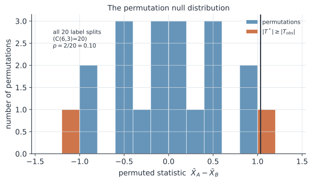
Two groups: treated $A=\{5.1, 6.3, 5.8\}$ and control $B=\{4.2, 4.9, 5.0\}$ . Observed statistic:

$T_{\text{obs}} = \bar{X}_A - \bar{X}_B = 5.733 - 4.700 = 1.033.$

There are $\binom{6}{3}=20$ ways to split the six pooled values into two groups of three. We recompute $\bar{X}_A - \bar{X}_B$ for each split and count how many give $|T^{*}| \ge 1.033$ (Figure 1). That count over 20 (with the continuity adjustment) is the two-sided permutation p-value. With small $n$ the smallest attainable p-value is bounded below by $1/20 = 0.05$ .

In code#

R#

set.seed(1)
a <- c(5.1, 6.3, 5.8); b <- c(4.2, 4.9, 5.0)
obs <- mean(a) - mean(b)
pool <- c(a, b); n <- length(a)
perm <- replicate(10000, {
  idx <- sample(length(pool), n)          # shuffle labels
  mean(pool[idx]) - mean(pool[-idx])
})
(sum(abs(perm) >= abs(obs)) + 1) / (length(perm) + 1)   # two-sided p

Python#

Python

import numpy as np
rng = np.random.default_rng(1)
a = np.array([5.1, 6.3, 5.8]); b = np.array([4.2, 4.9, 5.0])
obs = a.mean() - b.mean()
pool = np.concatenate([a, b]); n = len(a)
perm = np.empty(10000)
for i in range(perm.size):
    p = rng.permutation(pool)              # shuffle labels
    perm[i] = p[:n].mean() - p[n:].mean()
print((np.sum(np.abs(perm) >= abs(obs)) + 1) / (perm.size + 1))

0.0978902109789021

Julia#

Julia

using Random, Statistics
Random.seed!(1)
a = [5.1, 6.3, 5.8]; b = [4.2, 4.9, 5.0]
obs = mean(a) - mean(b)
pool = vcat(a, b); n = length(a)
perm = map(1:10_000) do _
    p = shuffle(pool)                      # shuffle labels
    mean(p[1:n]) - mean(p[n+1:end])
end
println((count(x -> abs(x) >= abs(obs), perm) + 1) / (length(perm) + 1))

Why it matters for statistics#

Permutation tests give exact or nearly exact p-values under minimal assumptions, relying only on exchangeability rather than normality or large samples. They are a robust, transparent alternative to parametric tests and generalize to almost any statistic you can compute.